August 30, 2026 · Lecture · LibreTimes
Machine Learning 1. Lecture 5. The Support Vector Machine
Contents
- What this lecture is about
- The problem statement: approximating and regularizing the empirical risk
- The optimal separating hyperplane
- The Karush–Kuhn–Tucker conditions
- Applying it to the SVM problem
- Support vectors and the types of objects
- The dual problem
- Kernels and rectifying spaces
- The kernel trick
- How to choose the constant C
- SVM as a two-layer neural network
- Advantages and drawbacks of SVM
- SVM regression
- Regularization for feature selection
- Elastic Net SVM
- Support Features Machine
- The relevance vector machine
- Summary
- Seminar
What this lecture is about
A rather mathematically dense lecture — about a very interesting method, the support vector machine (SVM). If you ask what the three strongest machine learning methods are, the answer has stayed the same for a couple of decades now: support vector machines, boosting over decision trees, and neural networks. One of this trio is the subject of today's lecture.
We will discuss the problem of building a linear classifier, talk a little about how to adapt the same methods to regression, and, in the third part, about non-standard regularization methods for SVM-like methods.
The problem statement: approximating and regularizing the empirical risk
Definition (The problem of training a linear classifier). Given: a training sample , where are the objects, vectors from the set , and are the class labels, elements of the set .
Find: the parameters , of the linear classification model
Criterion — the minimum of empirical risk:
where is the margin of the object .
The objects are described by numerical features, and is the known correct answer, «yes» or «no». When we built the linear classifier as a model of a neuron by the stochastic gradient method, we got rid of the free term : we said there is a constant feature always equal to , added it to the vector as the th coordinate, and put as the th coordinate of the vector . In SVM, on the contrary, it is not got rid of, and as we go you will understand why: an additional constraint will be imposed on that makes no sense to impose on . Different methods treat the free term differently.
What follows is so far a reminder. The empirical risk, the number of errors of the model on the training sample, is inconvenient: it is a piecewise constant function of the parameters and . The margin is in effect the signed distance from the point to the separating hyperplane; if it is negative, there is an error on the object. Let us replace the threshold loss with an upper bound — piecewise linear but continuous: one minus the margin, with positive truncation.
Definition (Approximating and regularizing the empirical risk).
- Approximation penalizes objects for approaching the class boundary, increasing the gap between the classes.
- Regularization penalizes unstable solutions in the case of multicollinearity.
The piecewise-linear loss and the threshold loss (slide).
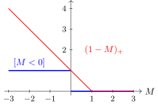
The threshold loss (blue) and its piecewise-linear upper bound (red). On the stretch there is no error yet, but the object is already penalized for approaching the class boundary.
Let me note an interesting property of this loss function. On the stretch from zero to one there is no error on the object yet, the margin is positive, but the object begins to approach the boundary between the classes, the separating surface, and we start penalizing it for that. This turned out to be a very important property. It is not just an approximation of the threshold function by which we replace the problem of minimizing the number of errors with one more convenient for optimization. The replacement cannot be called dishonest; on the contrary, it is very good and right: an additional principle is introduced — that objects should stand farther from the separating surface.
That is not all. We apply one more principle, which we have also covered already: linear models suffer from multicollinearity, overfitting can be the consequence, and an indirect sign of it is, in the jargon, the coefficients of the vector running off to plus or minus infinity. To prevent this, we pull the vector towards the origin: this is regularization, because the Euclidean, norm of the vector is minimized. In effect two functionals have been introduced: the main one, the approximated empirical risk, and a second one — among all the solutions that minimize the first, if there are many, choose the one with the minimum norm.
This statement is in effect already the support vector machine. To bring out and study its interesting properties, let us carry out another, alternative formalization of the problem — a little more complicated, but more geometric and intuitive. It will lead us to a better understanding of what a support vector is and where it comes from here.
The optimal separating hyperplane
Let us make, literally for one step, an additional assumption that we will get rid of later: the sample is linearly separable. That is, there is a hyperplane that separates the sample into two classes without errors. Algebraically: there exist a direction vector and a translation given by the scalar parameter for which a system of inequalities holds — one per object:
This system can be normalized. The parameters and enter it linearly, so if all the inequalities are multiplied or divided by the same positive scalar, the system does not change. Let us use the freedom of normalization so that the minimum margin equals one: find the minimum left-hand side and divide all the inequalities by it.
Now let us introduce the optimality principle for the separating hyperplane: build it so that the separating strip between the classes has maximum width. The separating strip is the locus of points at which the discriminant function lies in the range from minus one to plus one; there are no sample points in it, and the separating hyperplane passes through the middle:
I claim: if we choose a direction vector for which the strip is as wide as possible, then its boundary hyperplanes necessarily rest against some points of the training sample, and on one side against an object of class , on the other against an object of class :
The proof is very simple: if we choose a strip of the maximum possible width at which the sample is still separated without errors, and on one side the strip has not yet rested against anything, then it can be widened until it does. There is no error on these two objects, and they lie exactly on the boundary of the strip.
The width of the strip is computed from these conditions. Project the difference onto the unit vector — unit length is not guaranteed for , so we divide by the norm. Expand and ; the cancel:
The separating strip, the support objects , and the vector (slide).
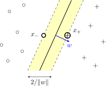
The separating strip of maximum width (yellow); the separating hyperplane is in the middle. The strip rests against the objects and of different classes lying on its boundaries; is the direction vector, and the width of the strip is .
We have derived a very interesting relation: the width of the strip is divided by the Euclidean norm of the direction vector of the separating hyperplane. So the principle of maximizing the width of the separating strip is nothing other than regularization! An unexpected result: it would seem, what connection could there be between them, and yet it turns out to be direct, and regularization in the linear classification model has a geometric interpretation.
But we did all this assuming the sample is linearly separable. In practice that is rather an exotic case, when the training sample divides perfectly into two classes without errors — it happens rarely. Let us lift this restriction, having worked out the geometry and understood how it leads algebraically to the problem statement. Whether to minimize the norm or its square makes no difference; the square is more convenient, as we will see in a moment.
Definition (Justifying the piecewise-linear loss). A linearly separable sample:
Moving to a linearly non-separable sample (a heuristic):
The equivalent unconstrained minimization problem:
What is inconvenient about the first statement? If the sample is linearly non-separable, the system of inequalities is inconsistent, and we minimize the criterion over an empty set: the problem has no solutions. The inequality constraints must be relaxed. Let us introduce additional non-negative variables — slack variables. This is in effect a penalty for violating an inequality: yes, the inequality may fail to hold, and how much it fails is . We would like the total violation of the inequalities to be as small as possible, so an additional functional is introduced into the criterion. We get a two-criterion problem: on the one hand, widen the separating strip as much as possible; on the other, minimize the total penalties for objects that jump the boundary of the strip and end up inside it or even in the other class. We want to minimize both criteria and add them with the coefficient . What it equals we do not know yet — it will apparently have to be chosen; more on that later. In multi-criteria optimization this way is called scalarization of criteria, and it is probably the most frequently used in practice: we add the criteria with some coefficients and get a separate headache — how to choose these coefficients.
This is a mathematical programming problem: minimizing a functional under inequality constraints, where the constraints are linear and additional variables have appeared. They can be got rid of very simply. From and it follows that . We minimize over among other things, and if is bounded from below by some function, it is always profitable for us to take equal to that function. Substituting, we get rid of and obtain an unconstrained minimization problem — the very one we wrote out at the very beginning: approximation of the empirical risk by a piecewise linear continuous loss plus regularization.
So the two statements are equivalent. One is unconstrained minimization. The other is derived from the geometric principle of the maximum width of the separating strip and written as a mathematical programming problem. In it the functional is quadratic in and linear in , the constraints are linear — it is a quadratic programming problem. Classically it is this one that is solved, because its solution gives an understanding of very important additional properties of the method.
Remark (Why). Someone asked why carry the constant along. We are about to differentiate with respect to , and the will cancel the two from the exponent — a purely technical convenience. In general we are entitled to apply any monotonic function to the functional being optimized, and the solution will not change; that is why the norm was squared and multiplied by .
The Karush–Kuhn–Tucker conditions
How to solve optimization problems under equality and inequality constraints is usually covered in courses on numerical optimization methods; it is not the subject of our course. Here is a reminder, and we will use this recipe purely as consumers. It can be found word for word in this notation on Wikipedia, and we will need it more than once.
Theorem (The Karush–Kuhn–Tucker conditions). The mathematical programming problem:
Necessary conditions. If is a local minimum point, then there exist multipliers , , and , , such that
The functions , , are smooth — linear, quadratic, anything at all, as long as they are smooth. If there were no constraints, we would simply differentiate and set the derivative to zero. With constraints the recipe generalizes: we form the Lagrange function — a weighted sum of all the functions , and with Lagrange multipliers; for us these are additional variables. We differentiate the Lagrange function and set the derivative to zero, not forgetting to include the original constraints in the system. The dual variables corresponding to the inequality constraints are non-negative — these are the dual constraints. And the last, most exotic condition is the complementary slackness condition: either or the inequality constraint holds as an equality.
Applying it to the SVM problem
Let us put our quadratic programming problem into the recipe. I omit half a line of calculation and write the Lagrange function straight away:
are the variables dual to the constraints (there are as many of them as objects in the sample); are the variables dual to the constraints . The Karush–Kuhn–Tucker conditions:
Differentiating is easy: the Lagrange function is quadratic in and linear in all the other variables.
The first equation immediately expresses through the dual variables: the direction vector of the separating hyperplane is a linear combination of the original vectors . Moreover, , and because of the complementary slackness condition some may turn out to be zero. So the main parameter of the model is a linear combination of only some objects of the training sample. These we will call support vectors, and the solution does not depend on the other objects at all. This interesting property is visible literally in the first steps.
From the third equation: is a positive constant, and and are non-negative. Hence all the are bounded: the dual variables live in the -dimensional cube . One can see that the whole solution is expressed through , and one wants to get rid of all the variables except .
Support vectors and the types of objects
Let us bring the system of conditions together:
Definition (Support object). An object is called a support object if .
But that is not all that can be said. Objects fall into three types depending on the value of : the left end of the interval , the right end, or somewhere strictly in between.
Definition (The types of objects).
- ; ; ; — a peripheral object.
- ; ; ; — a boundary support object.
- ; ; ; — a violating support object.
- . Then , since together they make ; so , and by complementary slackness , whence the margin . The object lies inside its class and in general does not fall on the boundary of the separating strip. We call such an object peripheral: does not depend on it; it can in principle be thrown out and nothing will change.
- . Then is also strictly between zero and , so ; and since , the margin constraint holds as an equality: . The object lies exactly on the boundary of the separating strip — these are the objects the strip rested against when we widened it by the optimality principle. Let us call it a boundary support object: support, because and the position of the separating hyperplane depends on it; boundary, because it is exactly on the boundary of the strip.
- . Then , : we penalize the object for crossing the boundary and ending up inside the strip or even in the other class; its margin is less than one. This is a violating support object.
It turns out that the support objects are those that lie on the boundary of the separating strip or fall inside it. And this we no longer much like: objects that have flown off into the other class are objects with an error, and the solution depends on them too. What if it is an outlier on which, say, we wrongly specified , and it simply flew off into the other class? It ought to be thrown out altogether, yet we use it substantially in the solution, and the separating hyperplane rests on it. A weak spot of SVM: noise outliers, objects with too large a negative margin, also turn out to be support objects. That is how the problem statement came out; nothing can be done.
The dual problem
Now let us make a dual problem out of the system of conditions, getting rid of all the variables except . is expressed through ; can also be expressed — from the equations for objects with margin equal to one; , can also be got rid of. What remains is a problem depending only on the dual variables. The substitution is completely routine, two lines of trivial calculation, and I will not tire you with it.
Definition (The SVM dual problem).
The solution of the primal problem is expressed through the solution of the dual one:
A linear classifier with the features :
Again a quadratic programming problem, now in : the functional depends on the pairwise products and linearly on . The constraints: lives in a cube with edge along all coordinates, and the equality defines a hyperplane. We get the intersection of a hypercube and a hyperplane in the space , where is the size of the training sample. We minimize a quadratic functional, a convex function, over a convex set, and the solution is unique. This is a very good property.
There are numerical methods that find this solution quite efficiently. General methods solve any quadratic programming problem, but this problem is specific: the constraint is a section of a hypercube by a hyperplane. And it is also sparse. If the problem is solvable in principle, we will build a separating hyperplane that makes few errors; then most objects will be peripheral, and only a small share of the objects will get nonzero . Sparsity is also very good for special numerical methods. They were well developed some 20–25 years ago, there are a huge number of implementations, and they are in ready-made libraries. Telling even one method in full detail would be a separate lecture; let us assume we can solve the dual problem. The rest is clear: from the found we express , find from the condition for any boundary support object, and build the linear classifier.
Let us substitute into the classifier — and see what interesting thing has come out. In place of we substituted a linear combination with coefficients , and the scalar product turned into a sum of scalar products. The classifier was linear with parameters and has remained linear with parameters . Only now there are not parameters, as many as there were features, but , as many as objects in the training sample. And all the objects that are not support objects can be thrown out, and most likely very few objects will remain, with the scalar products acting as features. This is very similar to prototype selection in metric classifiers. We have in effect kept the support objects in the training sample and compute a measure of closeness to them as features — here not yet a metric but another measure of closeness, the scalar product.
Kernels and rectifying spaces
An even more interesting point. Note: in the dual problem our original data, the x's, enter only through pairwise scalar products, and in the classifier itself too. The features are not used anywhere else. Recall the lecture on metric methods: sometimes it is easier to measure some closeness between objects than to compute their features. Perhaps scalar products too can be obtained somehow bypassing features? And can we replace the scalar product of vectors by some other function of a pair of objects? That would give enormous freedom. If the function is not the ordinary scalar product but something more complex, depending nonlinearly on the objects, then we will build a nonlinear separating surface. The linear classifier can be generalized and made nonlinear!
Definition (Kernel). The idea: replace with a nonlinear function . A transition to a rectifying space, as a rule of higher dimension: .
A function is a kernel if for some , where is a Hilbert space.
When can this be done? Obviously, when the function of a pair of objects behaves as a scalar product in some new space, into which we have moved by some, in general nonlinear, transformation . The new space has a scalar product, it is Euclidean; let us generalize as far as possible and say it may even be a Hilbert space, that is, of infinite dimension. Why is this possible? Because from the very beginning we could have taken as the feature descriptions of objects not but , and nothing would have changed: we would have got the same optimization problem, moved to the dual one in the same way and solved it in the same way, only everything in the new space . There we still build a linear separating surface, which is why it is customarily called rectifying.
Is every function of a pair of objects a scalar product in some space after some transformation? No, not every one: the freedom to choose kernels is limited.
Theorem (Mercer). A function is a kernel if and only if it is
- symmetric: ;
- non-negative definite: for any .
Symmetry is clear: a scalar product must be symmetric, there is no getting around it. The second condition is rather hard to check: for some functions it can be proved relatively easily, and for some it is a difficult problem. What to do in that case? The trick is this: prove mathematically that certain transformations make new kernels out of kernels, and then a kernel built by such transformations is guaranteed to be a kernel by construction. The list is far from complete, but it is quite enough for the kernels used in practice; everything else is such an exotic thing that it will be hard even to find publications on it.
Proposition. Constructive methods of synthesizing kernels:
- is a kernel;
- the constant is a kernel;
- the product of kernels is a kernel;
- the product is a kernel;
- with is a kernel;
- , if is a kernel, then is a kernel;
- if is a symmetric integrable function, then is a kernel;
- if is a kernel and the function can be represented as a convergent power series with non-negative coefficients, then is a kernel.
The scalar product is a kernel by definition; a constant is a kernel. That a product of kernels is a kernel is easy to verify by substituting into the definition with integrals. In item 4, is a single feature, and is a scalar product in a one-dimensional space. A sum of kernels is a kernel, but only with positive coefficients; with non-positive ones, generally speaking, not. In item 6 we take any transformation of the original -dimensional vectors into new -dimensional vectors and substitute the result into a kernel, the scalar product for example. Incidentally, the square of a kernel is a kernel, and so is any natural power of a kernel. Item 7 is an integral convolution; I will not prove it; such things are proved in courses like the equations of mathematical physics. Item 8: a new kernel can be obtained from a kernel by applying a function to it, but far from any function — only in rare cases. Two examples of series with non-negative coefficients: the exponential, all of whose Taylor coefficients are positive, and the sum of a geometric progression . There are rather few such functions. These eight rules, applied in arbitrary order one after another, are enough to generate a huge heap of kernels.
Example (The rectifying space for the quadratic kernel). Let , , where , . This is a kernel: the square of the scalar product is a product of kernels.
Problem: find the space and the transformation for which .
Let us expand the square of the scalar product:
Thus , : the same transformation is applied to and to , and it makes three new features out of two original ones. A linear surface in the space corresponds to a quadratic surface in the original space .
The same exercise can be done for vectors in and for powers greater than two — the same calculation, only somewhat more cumbersome.
Example (Examples of kernels).
- The quadratic kernel, : .
- The polynomial kernel with monomials of degree , : .
- The polynomial kernel with monomials of degree : .
- A neural network with sigmoid activation functions: , .
- A radial basis function network (the RBF kernel): .
For and the square of the scalar product, the dimension of the rectifying space is quadratic in . For the power , the transformation forms from the features all possible products of degree — monomials, and the dimension of the Hilbert space is the number of such monomials. And if we want to move from linear separating surfaces to arbitrary polynomial ones, with monomials of all degrees from zero to ? It turns out to be very simple and elegant: take . Multiplying out the brackets, we get all possible monomials not only of degree but of all lower degrees, because a certain number of ones will enter the products.
The kernel trick
Here is a remarkable fact. The original dual problem, which we solve numerically, depends on the data only through the matrix — the Gram matrix, the matrix of scalar products between all the objects of the training sample; also through , but that does not depend on the features. We form this matrix, feed it to the numerical method, and it gives the solution in the dual variables . If we were building a linear separating surface in the original space, is just the scalar product. Now let us take the Gram matrix, add one to each of its cells and raise it to the power , nothing more. Feed the transformed matrix to the same dual problem solver. The obtained are now the coefficients of a solution that builds a polynomial separating surface in the original space. This corresponds to solving a linear problem in a space of much higher dimension; one can even compute which — the number of combinations summed over all powers from zero to .
A very beautiful technique that makes computation practically no more expensive. We solve the same problem we would solve for a linear separating surface, and an elementary elementwise transformation of the Gram matrix lets us build a polynomial surface instead of a linear one. This is the kernel trick: a very simple operation on the matrix of scalar products seriously extends the class of separating surfaces.
If we take the kernel , we in effect build a two-layer neural network: the first layer computes scalar products, the kernel function plays the role of the activation function, and the second layer is a scalar product with the coefficients . Another useful construction is the radial basis function network. It resembles a metric classifier: the «scalar products» are computed as a Gaussian closeness function over the Euclidean metric. So by choosing the kernel, a linear classifier can be made into a polynomial one — one, a two-layer neural network — two, a radial basis function network — three. And if we take some other kernels — imagine what freedom of choice and what flexibility in building separating surfaces!
On a two-dimensional model problem this variety can be seen. The linear kernel gives a straight line in the original space. There is a point here that is classified with an error: the sample is linearly non-separable. A polynomial kernel of degree 3 builds a surface such that the sample becomes separable in the rectifying space. The Gaussian kernel gives an even more flexible surface.
How to choose the constant
Let us return to the postponed question: what does the constant with which we weighted the two criteria affect? In the notation one sees: if is large, the factor is small, we do not strive much to maximize the width of the separating strip — weak regularization, and there are few support objects; in the example there are three. If we decrease , that is, strengthen the regularization, we strive to widen the strip. But where can it be widened if there are errors in the sample anyway? More and more objects with a margin less than one become support objects: the strip widens and they fall inside it. Note also how the position of the separating hyperplane changes along the way.
Optimization over a grid is usually recommended: solve the problem for different values of — incidentally, there are efficient methods that solve the problem simultaneously for many , given by a grid for example — and choose the at which cross-validation, leave-one-out or hold-out, is better. is a hyperparameter that is convenient to choose, for example, by hold-out: split the sample into training and test and see at which the test gives the best solution.
SVM as a two-layer neural network
What I have already said in words about the kernel written as a neural network: in fact a two-layer neural network can be discerned in any linear classifier written through a kernel in the dual space. Let us renumber the objects so that are the support ones:
SVM as a two-layer neural network (slide).
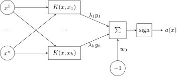
SVM as a two-layer network: instead of scalar products the first layer computes the kernels to the support objects — the weights of the first layer are the support objects themselves; the second layer is a linear combination with coefficients and threshold .
Initially we have a vector in . First we take its scalar products with vectors — not with all the training ones, only with the support ones: is the number of support objects, and the fewer there are, the simpler the network. This is the number of neurons in the hidden layer, and the neurons of the hidden layer compute closenesses between the object being classified and the support objects. The second layer is a linear combination with the coefficients given by the numerical optimization method. If is the scalar product, we get a single-layer perceptron, a linear classifier. And if is a nonlinear function, a scalar product in the rectifying space, we get a two-layer network. That is, SVM is a way of implementing two-layer neural networks of a certain kind together with a method of training them. And if the kernel is radial, depending on the norm of the difference of two vectors, it is a metric between objects, and SVM is also a metric classifier based on computing closenesses, with automatic built-in prototype selection at that. Only here they are called not prototypes but support vectors; the meaning is the same.
Advantages and drawbacks of SVM
That is the whole main, textbook story about SVM. Let us sum up.
Advantages of SVM over two-layer neural networks:
- the convex quadratic programming problem has a unique solution. It could also be solved by the stochastic gradient method, as in the previous lectures, but numerical quadratic programming methods make it possible to find the support vectors faster and, above all, exactly — and so
- the number of neurons in the hidden layer is determined automatically: it is the number of support vectors. And that very unique solution is found along the way. This is of course better than general-purpose stochastic gradient for any neural networks whatever.
Drawbacks of classical SVM:
- noise objects (outliers) are support objects;
- there are no general approaches to optimizing the kernel for a problem — this is still an unsolved theoretical problem: there is much research but no final answer;
- on big data SVM trains more slowly than stochastic gradient, even with efficient quadratic programming methods tailored to SVM. So on very big data something SVM-like with kernels is better done by neural network methods;
- there is no «built-in» feature selection;
- the constant has to be chosen — additional tedious technical work.
SVM regression
We will have occasion to talk about loss functions in regression in more detail; for now, briefly. Usually regression uses least squares with the quadratic loss. But if we replace it with a piecewise linear function that does not penalize small deviations of the prediction from the correct value, we get a quadratic programming problem similar to SVM.
Definition (SVM regression). The regression model: , , . The loss functions: and , where .
The problem statement:
The change of variables , reduces it to a quadratic programming problem:
Here too there is a margin-like functional with positive truncation, and slack variables are introduced, but now there are twice as many: we penalize an object for jumping out of a tube around the function being approximated — either upwards or downwards, and that has to be penalized separately. Otherwise this too is a quadratic programming problem with linear inequality constraints; the solution is also unique, also expressed through support vectors, and the replacement of scalar products in the dual problem by a kernel is also possible. Originally it is trivial linear regression, but with the kernel trick it can be generalized to nonlinear regression models.
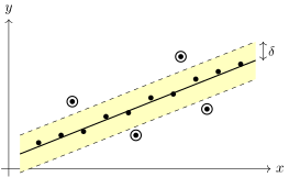
SVM regression: a tube of width around a linear function. Deviations inside the tube are not penalized; the points that jumped out of it upwards or downwards (circled) turn out to be support objects.
The tube is the analogue of the separating strip between classes in classification, and the support objects turn out to be the points that jumped out of the tube downwards or upwards.
Regularization for feature selection
I also wanted to talk about regularization. Did we have to use regularization? We got the optimality principle — the maximum width of the separating strip — through the Euclidean, norm. And if in the problem statement we replace the norm with the norm of the coefficients ? A very interesting effect results, and a generalization is immediately visible. This is an important point.
Our loss function is continuous but not smooth: piecewise linear, with a kink at the point . Thanks to this kink an optimization problem with inequality constraints appeared. The Karush–Kuhn–Tucker conditions led to some inequalities holding as equalities, and that led to support objects. The appearance of support objects is due to the non-smoothness of the loss function: were the loss smooth, there would be no additional inequality constraints, the KKT conditions would not be needed, and support objects would not appear. And if non-smoothness is put into the regularizer, it becomes profitable for many coefficients to become zero: constraints have to be imposed on them, which through the KKT conditions lead to many finding it profitable to take the value zero. And a zero is nothing other than feature selection.
Definition (1-norm SVM (LASSO SVM)). Approximation of the empirical risk with regularization:
Bradley P., Mangasarian O. Feature selection via concave minimization and support vector machines. ICML 1998.
The regularization parameter plays a role called selectivity: the larger , the more features get zero coefficients and the fewer of them remain in the model. This appeared in the literature in at least two different works: some authors called the method 1-norm SVM, others LASSO SVM. LASSO is in general the name of the regularization method: it is a lasso, a noose that we throw over the coefficient vector, and by tightening it with the selectivity coefficient we force the vector to give up excess degrees of freedom. It is a poetic metaphor from cowboy films about the Wild West. And it stands for Least Absolute Shrinkage and Selection Operator: the method of least absolute values, an analogue of least squares. We shrink the coefficient vector, and this leads to feature selection: some coefficients become zero.
The method also has a drawback: too aggressive feature selection. As the selectivity grows, significant features begin to be thrown out too, while not all the excess, noise features have been thrown out yet. This was found in experiments on model data: a number of significant features on which depends linearly are built into the dependence, and noise features on which does not depend are added. Synthesizing such data is not hard, and we know in advance which features are informative. Is it true that as is increased smoothly, the method first throws out the noise features and then gets to the informative ones? It turned out — not true: some informative features begin to be thrown out too early. And we would like all the significant features on which depends to gather together and stay in the model, to group — even though there may be linear dependences among them and it may be profitable to throw some of them out. regularization is not able to provide such grouping. The method is interesting but needs refinement, and refinements began to appear.
Why does the regularizer lead to feature selection? Non-smoothness causes problems in solving the problem; can the functional be brought to a smooth form? It can, by a change of variables:
For one original variable we introduce two new ones, both non-negative: if is positive, it is expressed through ; if negative, through ; and one of them is always zero. The absolute value is expressed not by a difference but by a sum. We get a smooth problem:
The absolute value has disappeared, the problem in , is smooth — it is a generalized SVM with additional inequality constraints. Again we apply the Karush–Kuhn–Tucker conditions and see: the larger , the more indices for which ; but then , and the feature is not taken into account. I have shown this as an idea, without the details of the proof.
Example (Comparing and regularization). The cancer diagnosis problem (prostate cancer) from the UCI repository, eight features; the curves are the coefficients of the features as functions of the regularization parameter. As all features are zeroed. As decreases, degrees of freedom appear, new features come in, and more and more features enter the model with nonzero coefficients. There is nothing of the kind with regularization: the original, classical regularization of SVM does not allow feature selection.
T. Hastie, R. Tibshirani, J. Friedman. The Elements of Statistical Learning. 2001.
Elastic Net SVM
Can the two regularizations be combined? Then both and have to be used.
Definition (Doubly Regularized SVM (Elastic Net SVM)).
Li Wang, Ji Zhu, Hui Zou. The doubly regularized support vector machine. 2006.
The method is called doubly regularized: the sum of two regularizers, and , is used. Why do they work so well together? We weaken the selectivity, , and capture a few more features than LASSO, which selects them too harshly. And on the remaining features we remove the effects of multicollinearity with regularization. That gives that very grouping effect: if depends on features, they are selected together, even if they are linearly dependent on each other.
But, as a series of subtle experiments on model data showed, if the model has informative features and many noise features on which does not depend, the noise ones may also group and enter the model together. That is quite bad: as the selectivity is gradually increased, it may turn out that grouped noise features stay in the model while some really useful, informative features, also grouped, are thrown out. Besides, two regularization parameters have to be chosen.
Support Features Machine
Can we make informative features group together while noise features are thrown out individually? It turns out we can, but differently, not as in Elastic Net: and are combined in a single regularizer.
Definition (Support Features Machine (SFM)).
Tatarchuk A., Urlov E., Mottl V., Windridge D. A support kernel machine for supervised selective combining of diverse pattern-recognition modalities. 2010.
With such a regularizer there is the selectivity effect, that is, feature selection, and the effect of grouping informative features: significant interdependent features () group and enter the solution jointly, as in Elastic Net. And noise features () do not group and are suppressed independently of each other, roughly as in LASSO. There is only one regularization parameter. This is a nontrivial invention, but a rather exotic method: it requires non-standard optimization procedures that are not so easy to find. In principle this has been done; one can look in the papers.
The relevance vector machine
I will mention in a couple of words a quite exotic machine — the relevance vector machine (RVM). Here too a classifier linear in the dual variables is sought, as in SVM, but separately the aim is set that the maximum number of become zero — that the solution be even sparser than in SVM. The regularization is imposed not through the norm on but as a constraint on . It is an exotic variant of an SVM-like method with a different regularization and even more interesting sparsity properties.
M. E. Tipping. The relevance vector machine. 2000.
Summary
- SVM is the best linear classification method, thanks to its loss function penalizing objects for approaching the separating surface, increasing the gap between the classes.
- A generalization astonishing in its elegance and simplicity is the move from linear classifiers to nonlinear ones. Not entirely arbitrary ones, because the choice of kernels is not entirely arbitrary, but very wide classes of separating surfaces are built simply by choosing a kernel — by transforming the Gram matrix, the matrix of scalar products between objects.
- SVM easily generalizes to regression problems too.
- Regularization increases the gap, removes multicollinearity and reduces overfitting.
- Non-smoothness of the loss function leads to selection of objects, non-smoothness of the regularizer to selection of features. The original data is a matrix whose rows are objects and columns are features. By choosing non-smooth loss functions we can arrange selection of rows, and by choosing non-smooth regularizers selection of columns. These are two, one could say, orthogonal techniques, and both are tied to non-smoothness. It took decades to understand how this works.
V. N. Vapnik, A. Ya. Lerner. Pattern recognition using generalized portraits. 1963 (in Russian). C. Cortes, V. Vapnik. Support vector networks. 1995.
Remark (How the dimension grows when moving to a kernel). After the lecture someone asked: how does the dimension increase when we apply a kernel? We replace the scalar product in the original space with another function of a pair of objects. But in the new space we move to there must exist a scalar product, and our function is precisely the scalar product in the space over the transformed vectors. The transformation is the computation of new features from old ones, and it can happen with an increase in dimension, since is a Hilbert space — up to infinity. A polynomial separating surface is when all possible products of the original features of degree at most , monomials, are taken as features. The dimension has increased greatly, but by solving a linear problem in the new space we build a polynomial surface in the original one. The general recipe is this: take the original features, build all possible functions over them — here imagination runs free, infinitely many can be built — and in the extended space build a linear classifier by the same SVM method. In the original space some nonlinear surface will correspond to it. In the example with the quadratic kernel we reduced it to the scalar product of two vectors of three coordinates, and the same transformation made three new features out of two original ones by multiplication.
No comments yet
Be the first to share your thoughts.