August 30, 2026 · Lecture · LibreTimes
Machine Learning 1. Bayesian Classification Theory
Contents
- What this lecture is about
- Bayesian classification theory
- The probabilistic formulation of classification
- The optimal Bayes classifier
- Empirical estimation problems
- The naive Bayes classifier
- The hypothesis that the features are independent
- Features with exponential-type densities
- The linear naive Bayes classifier
- A survey of Bayesian classifiers
- The Parzen window method
- The quadratic discriminant
- Fisher's linear discriminant
- Gaussian mixtures with diagonal covariance matrices
- The radial basis function network
- Conclusions
- Seminar
What this lecture is about
For most of today's lecture we talked about estimating the densities of probability distributions from a sample: parametric, nonparametric, and separating a mixture of distributions. The last third stands somewhat apart: we change the problem and talk about classification again, but we use this mathematical machinery to look at a class of methods that is new for us.
Let us recall the large classes of classification methods we have already covered: linear models; models that are nonlinear but based on the principle of separability and margin maximisation; metric classifiers; logical classifiers; compositions. With these we have covered practically all of machine learning. One large class of classification methods remains, called statistical. They are based on estimating probability densities — but now we will estimate the density within each class. Take all the objects of one class: their are all the same and can be dropped, and from these objects we estimate the density. We will see that if we can solve the density estimation problem for each class separately, we can also solve the classification problem in probabilistic terms.
Bayesian classification theory
The probabilistic formulation of classification
Definition (The probabilistic formulation of classification). are the objects, the classes, is a probability space with density .
Given: , a simple (i.i.d.) sample.
Find: with minimum probability of error.
Suppose the joint density is known:
- is the prior probability of the class ;
- is the likelihood function of the class ;
- is the posterior probability of the class .
By Bayes' formula .
The Bayes classifier:
We will assume that our sample is simple, i.i.d., and comes from some unknown joint density of and , and our task is to find a classification algorithm with the minimum probability of error. We can pose the problem this way if it is probabilistic from the start, that is, if we work from the outset in a probability space of pairs . Let us temporarily assume that the joint density is known — a temporary assumption; later we will drop it and estimate the densities from the sample. Then the conditional probabilities can be written out in two ways. They are equivalent, but the four constructions that appear here need a detailed explanation.
A convention: I will write discrete probabilities with a capital , and densities in a space that is as a rule infinite with a small . This is a mnemonic rule so that we recognise them easily. Our objects are very often vectors in , a continuous space, and densities in it are denoted by a small . The joint density of and is still continuous — although is discrete, is continuous — so it too is a small . So:
- is the density over the whole space , of all objects, regardless of which classes they belong to.
- : if we look at a particular object , we want to say which class it belongs to. This is, generally speaking, the most important quantity we have to estimate; it is called the posterior probability of the class. If we know the posterior probabilities, we can classify objects: assign to the class to which it belongs with the maximum probability. This is the maximum a posteriori principle — simple and seemingly obvious.
- is the prior probability of the class . It is very easy to estimate: if a stream of objects comes to us from this density, we look at what share of the incoming objects belongs to the class ; or we simply estimate from the training sample the share of objects of the class , a frequency estimate of the class probability.
- are the class densities themselves, the class likelihood functions, which we will model and estimate by the methods we have already discussed.
Please do not confuse these four quantities: they have completely different probabilistic meanings. For classification we need the posterior probability of the class at a given object , and thanks to Bayes' formula it can be written as the product of the prior probability and the class likelihood function, the density of the objects of the class. You may ask: where did I put , since we were supposed to divide by it? We do not need to: we take over , and does not depend on . is a pleasant function: any factors and terms that do not depend on can be removed from under it, and under we can take logarithms, which will also come in handy.
Remark (When the frequency estimate of the prior probability does not work). The frequency estimate of from the training sample does not always work, because sometimes the training sample was formed after filtering. For example, in problems with imbalanced classes: someone prepared a sample for us, originally there were a thousand times more objects of one class than of the other, the imbalance was evened out, and we were given a sample with equal numbers of objects of both classes. Then we must forget that such a sample can be used to estimate the prior class probabilities: the estimate will be wrong. We need to go to the person who filtered the data for us and ask what the share of the classes was in the rawest original data.
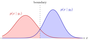
Classification by the maximum of the likelihood function with equal prior class probabilities, : an object is assigned to the class whose density at that point is larger; the separating surface is determined by how the class densities intersect (schematic).
A simple picture, a special case: if all are equal, the classification principle becomes very simple — we assign each object to the class whose density at the point is maximal. We only have to remember that in general we must also multiply by ; the picture just illustrates how classification happens and what the separating surface between classes can look like: it is determined by how these densities intersect.
The optimal Bayes classifier
There is a justification for this simple classification principle; moreover, it is optimal and is called the optimal Bayes classifier.
Theorem (The optimal Bayes classifier). Let and be known, and let be the loss from an error on an object of class . Then the minimum of the average risk
is attained by the optimal Bayes classifier
Remark 1: once the empirical estimates and are substituted, the Bayes classifier is no longer optimal.
Remark 2: the problem of estimating a probability density is harder than the classification problem.
I will not prove the theorem; it is proved in courses of mathematical statistics. If we know the prior class distributions and the class likelihood functions, and we have set the loss from an error on an object of class , then we can write down the expected loss — let us call it the average risk — and pose the problem of minimising it: what should the classification rule be so that the expected loss is minimal? Here is the loss , here is the law of total probability — a sum over all classes of the losses on the class — and the integral is the probability of an error on an object of class , when the algorithm gave a other than the right one. The theorem states that the minimum of the average risk is attained by that same Bayes classifier, with the one addition that was not there before: it includes , the loss from an error.
It turns out that the loss from an error on objects of class is the same kind of factor as the prior probability of class . We can, say, reduce the prior probability tenfold and increase the cost of an error tenfold, and the classifier stays the same: the losses from errors and the frequency of the class's objects trade off against each other, as it were.
And a couple of sardonic remarks. First: in fact this optimal Bayes classifier is not optimal at all. The theorem is derived under the assumption that the joint density of and is known, and in practice it is unknown: in practice we will estimate the densities from the sample. Then the Bayes classifier will no longer be optimal, will not minimise the expected error — it can overfit, like any normal classifier. Overfitting arises when we start estimating some model from a sample, and it does not matter whether it is a supervised problem, like classification, or an unsupervised one, like density estimation: when estimating a density we can already overfit. The phenomenon of overfitting is universal; it arises in any problem in which we optimise something on finite samples.
The second sardonic remark: it seems we are using a sledgehammer to crack a nut, because the problem of estimating a density is harder than the classification problem, and for two reasons at once. First, in classification we build a function that takes a finite number of values, while in density estimation we build a continuous-valued function; it seems we are solving an approximation problem in a richer class of functions, and that is probably harder. Second, in classification the main thing is to build the boundary between the classes, the separating surface. But when estimating class densities we care about the accuracy of the estimate everywhere: not only where the classes border on each other, but also on the periphery, where there is only one class, and we will chase a good estimate of the density on these peripheral objects too. Classification does not need this: classification is, after all, about building the boundary between the classes. These are the two reasons why density estimation, although a good technique, is somewhat heavy for classification. Nevertheless, a huge number of methods are built on it. And conceptually this is a very important understanding: density estimation and classification are closely interconnected, and when solving a classification problem we do, indirectly, estimate the distribution of the classes.
Definition (Two approaches to learning classification).
- Discriminative: are non-random vectors; is a classification model. Examples: LR, GLM, SVM, RBF.
- Generative: are random vectors; is a model that generates the data. Examples: NB, PW, FLD, RBF.
Bayesian classification models are generative: they model the shape of the classes not only along the boundary but over the whole space, which is excessive for classification; they need more data to train; they are more robust to noise outliers.
Empirical estimation problems
Definition (Empirical estimation problems). The frequency estimate of the prior probability:
Density estimates from the i.i.d. samples , :
- a parametric density estimate:
- a nonparametric density estimate:
- separating a mixture of distributions:
To build a classifier, we substitute estimates into the formula of the optimal Bayes classifier: the prior class probabilities by frequencies, and the class densities each from the objects of its own class, by any of the three methods we learned today. First we will look at one more important special case, and then we will carry out the substitution of all three.
The naive Bayes classifier
The hypothesis that the features are independent
One more important special case is the so-called naive Bayes classifier. Why naive? Because we assume that the features are independent random variables, and we specify one-dimensional densities of the features in each class. For this case we will now bring things almost to an analytical solution, and the solution will be very simple: the Bayes classifier with the independence assumption leads very easily to a ready formula with a very simple way of estimating, because the estimates are one-dimensional. Estimating one-dimensional densities, for each feature separately, is a much simpler problem than estimating multidimensional ones.
Definition (The naive Bayes classifier (Naïve Bayes)). The naive assumption: the features are independent random variables with densities , , .
Then the class likelihood functions can be written as a product of one-dimensional densities over the features, :
Taking logarithms under , we obtain the classifier
Estimating one-dimensional densities is a much simpler problem than estimating one -dimensional density.
The class likelihood function — the density of the objects in the class — factorises, since we have introduced the independence of the features: it is represented as a product of one-dimensional densities over the features. This at once gives a very simple analytical way of building the optimal Bayes classifier. Let us take logarithms of our probabilistic expressions under . We need to know a constant: the logarithm of the penalty for an error on an object of class plus the logarithm of the prior probability of the class. They are easy to obtain: we set the penalty ourselves, and the frequency of objects in the class can be estimated from the sample. And then an interesting construction: a sum of the logarithms of one-dimensional densities over each feature in each class.
Let us turn to these one-dimensional densities and estimate straight away: what if the density is Gaussian? This does not apply to every feature: a feature may be distributed nothing like a Gaussian. But if we assume that a feature is Gaussian, what do we need to know to estimate the parameters of the Gaussian distribution? Elementary: the mean of the feature and its variance. Two parameters, and , suffice to estimate a one-dimensional Gaussian distribution, and the estimate is different for each class. I have just proved, literally out loud, that this formula is not merely applicable: written here is a ready classification algorithm, a ready recipe and a ready procedure for training the naive Gaussian Bayes classifier from a sample. What do we need to do? Compute, for each feature in each class , the mean and the variance and substitute them here. That is all.
Features with exponential-type densities
But let us make this problem more interesting and consider a more general case: what if our features are not Gaussian? Recall that there is a wonderful thing called the exponential family of distributions. We have had it already, but in a completely different context: when we generalised multivariate linear regression to the case of non-Gaussian errors, the generalised linear model, GLM. There the least squares method turned into the maximum likelihood principle, and we used the exponential family to describe . Here the situation is different: we are describing classes, and we will use exponential densities to describe the distributions of the values of each feature separately.
Definition (Features with exponential-type densities). Assumption: the one-dimensional densities are exponential:
where , are parameters and , are function parameters.
The problem of maximising the log-likelihood
splits into independent subproblems for each pair :
In the problem is solved analytically, in not always.
Let us write out the formula. The most important thing in it is the exponential, which will let us apply the maximum likelihood principle: it cancels with the logarithm. The second important thing is linearity in : here we have the product of and the model parameter . These two features of the exponential density matter most. The density is defined up to an arbitrary function and an arbitrary function that does not depend on . The function parameters and we will of course fix, and the numerical parameters and we will tune by the maximum likelihood principle.
Let us write down the maximum likelihood principle. Strictly speaking we should have written a sum over all objects, a sum over all classes and then the logarithm; since the logarithm of a product turns into a sum of logarithms, a sum over all features appears. I have swapped the summation signs, taking the sum over the features and the sum over the classes outside, and inside there remains a sum over all objects of one class. These two outer sums show that the problem has decomposed completely, factorised: for each combination of a feature and a class there is a separate problem for the parameters and , which depend only on that feature and only on that class. That is the whole beauty of the independence assumption: we can estimate the parameters of all the distributions for each feature in each class separately. The problem splits into independent one-dimensional subproblems.
Example (Examples of exponential distributions). is the mean parameter, is the link function:
| Distribution | Values | |||||
|---|---|---|---|---|---|---|
| normal | ||||||
| Bernoulli | ||||||
| binomial | ||||||
| Poisson |
Let us look at the special cases. I have written them out once more, as in the lecture on GLM, when we talked about the various distributions that fall under the exponential family, because these are probably the most common cases of features of different types. If a feature is numerical, it can often indeed be considered approximately Gaussian; if not, other distributions have to be taken. The Bernoulli distribution is for binary features. The binomial is for integer features that have an upper bound. The Poisson distribution is for integer features without an upper bound, for example the number of clicks or the number of visits: such features, for which no definite upper threshold can be given, can be described by the Poisson distribution. And all these distributions are exponential — written here is in effect a proof of that fact: they just have to be written in exponential form. I draw your attention to the column with the inverse of the derivative — you will see in a moment why it is needed. And also to the fact that estimating the parameter in these special cases is easy: in the Gaussian case it is simply the variance, and in the others it is a constant that need not be estimated at all.
The linear naive Bayes classifier
Proposition. The solution for is expressed through the mean of feature in class :
The solution for cannot always be obtained from the equation , but for the Poisson, Bernoulli and binomial distributions ; for the Gaussian distribution (and if does not depend on ):
As a result, Naïve Bayes turns out to be a linear classifier:
where the terms are omitted if they do not depend on .
Now the most important part: the analytical solution of the maximum likelihood problem when all the features are independent and described by the exponential family. The solution takes one line. We take the log-likelihood functional for feature and class , set its derivative with respect to to zero, and immediately obtain: the derivative is numerically equal to the mean of feature in class . Look how everything worked out. The fact that does not depend on : its derivative is zero at once, dropped out, we no longer need it. Linearity worked: we took the derivative with respect to , remained, we summed — the mean of remained. Only the function gets in the way a little, but it entered here as a derivative, and to express the model parameter we have to take the inverse of the derivative and apply it to the mean.
Remember, I said at the very beginning: if the density of each feature in each class is Gaussian, we need to compute nothing but the mean and the variance. Now we have derived this in a much more general form, and this lets us use in the naive Bayes classifier not only Gaussian features but features of different types, including discrete-valued ones that certainly cannot be considered Gaussian. It turns out that a very small addition is needed for this: having computed the mean of the -th feature in class , apply the known function . Let us look at the table again: the most interesting thing is that only in the Gaussian case this function need not be applied, while in all the others it is some definite function — for discrete-valued features, for example, logarithms have to be computed. There is no great complication: we still have to compute the mean, and if the distribution is Gaussian, also the sample estimate of the variance of the -th feature.
And the most interesting thing: the naive Bayes classifier turns out to be a linear classifier (if the terms do not depend on the class — for example, for Gaussian features with a variance common to all classes). This is perfectly clear from the expression for the logarithm of the density: the value of the feature is multiplied by some coefficient , and we have just derived the formulas by which this coefficient is computed. That is, it is a linear classifier with a very simple learning method: its coefficients are computed from the means of the features and, if necessary, from the variances — dividing one by the other. Each feature is processed separately. There is also the quantity , through which the intercept is computed. But recall the lecture on classification quality, the ROC curve and the area under it: in a two-class problem the AUC does not depend on the intercept. The intercept is needed only to balance the errors of the first and second kind, to choose a point on the ROC curve, while the quality of the model as a whole is determined by how we found the coefficients .
For your collection, one more way of building linear classifiers. It is, of course, the worst of all known linear classifiers, because it is based on the naive assumption that the features are independent. But it is the fastest: no matrices need to be inverted, nothing; the coefficients are computed insanely simply, just from the means of the features.
Remark (Where and come from). The functions and are determined by the type of distribution you have chosen to describe the given feature. I gave four special cases, but believe me, there are a great many of them; even on Wikipedia you can see which distributions belong to the exponential family. This means that you can work easily and simply with features of different types: you only have to decide which density adequately describes the values of the given feature. This is of course a very big advantage of the approach. But let us not forget its biggest drawback, the independence assumption.
Very often, packages that implement the naive Bayes classifier implement only its Gaussian version: when estimating the densities of the individual features, only the mean is computed. And the fact that, depending on the exponential form of the feature's density, the mean has to be passed through the function is often forgotten. This is a rather subtle point: if your features are, for example, integer or even binary, do not use implementations of naive Bayes in which the mean of a feature is used without this correction.
A survey of Bayesian classifiers
The last thing I would like to do today is to take the optimal Bayes classifier, take all the density estimates we have looked at today, and simply substitute them to see what comes out. We have three ways of estimating a density, and we will substitute them in turn.
The Parzen window method
Definition (The Parzen window method (Parzen Window, PW)). The Parzen–Rosenblatt nonparametric density estimate with a distance function for each class :
The Parzen window method is a metric classifier:
Remark 1: the normalising factor cancels under if it does not depend on and .
Remark 2: the problems of choosing the kernel , the window width and the distance function remain.
First let us substitute the Parzen–Rosenblatt nonparametric density estimate into the formula of the optimal Bayes classifier. What do we see? First, hurrah: the normalising factor cancels — that terrible integral that causes difficulties in estimating multidimensional densities. It simply leaves the formula under : the is over , and must not depend on .
And here is an important point, in which it is very easy to get confused and do serious harm to classification quality. Imagine you are classifying an object : you compute this construction for each class at the point , that is, you compute the density. If you use a variable window width and estimate the class densities independently of each other — or not even a variable one, but simply choose the window width separately for each class — will not be able to cancel. Hence the conclusion: the window width must be chosen not for each class separately, but for all classes at once. Then will not depend on ; only then will it cancel, you will not have to compute these integrals, and only then will the formula be correct. This small detail is sometimes forgotten: "let us estimate the density for each class separately". Here is the rake it is easy to step on: if at the point the densities for different classes are estimated differently and each class has its own window width, you will not be able to use this formula of the optimal Bayes classifier; you will have to compute the normalising factors.
And second: we have already discussed this method, when we talked about metric classifiers, only we arrived at it differently — through nearest neighbours, through the wish to take the distances to the objects into account; we made a couple of generalising steps and wrote exactly the same formula. And now we know that this is not just a formula but a statistically justified technique: first, it is an estimate of a probability density, and second, it is the optimal Bayes classifier.
The quadratic discriminant
Now the parametric approach. We have already talked about parametric density estimates for the Gaussian distribution; let us substitute them. Each class has an -dimensional Gaussian density with centre and covariance matrix : each class has its own centre, its own expectation, and its own shape, the scatter ellipsoid. The scatter ellipsoids can be completely different: oriented differently, facing different directions, rotated differently relative to each other, and we want to describe their shape by covariance matrices.
Theorem (The quadratic discriminant (Quadratic Discriminant Analysis)). Hypothesis: each class has an -dimensional Gaussian density with centre and covariance matrix :
- The separating surface defined by the equation is quadratic for all .
- If , the surface degenerates into a linear one.
The quadratic discriminant is a plug-in algorithm:
The theorem is given without proof, but it can be proved out loud. The first thing it states: the separating surface is quadratic. The separating surface is the locus of points in the space where the expression under is the same for two classes. Take logarithms of the left- and right-hand sides of the equation: the exponential and the logarithm annihilate, and what remains is a quadratic form in in the numerator, while the denominator holds what does not depend on . We have just proved that the separating surface is quadratic for any pair of classes. Let us see what the quadratic term of this form is: multiplied by the inverted covariance matrix of the class, multiplied once more by . And what if the covariance matrices of the two classes between which we consider the separating surface turn out to be equal? Then the quadratic terms in this equation cancel too, only the linear ones remain, and the surface becomes linear.
That is, if in the optimal Bayes classifier we assume that the classes have Gaussian distributions, and additionally assume that the covariance matrices of the classes are the same — the scatter ellipsoids are the same and located in different places of the space, with different expectations, as if the classes were obtained from one another by a parallel translation — then the surface, quadratic in general, degenerates into a linear one, and we get one more linear classifier for our collection. It is called the linear discriminant, and the general one the quadratic discriminant. We know how to estimate covariance matrices and expectations from a sample, so this is simply a ready recipe.
Fisher's linear discriminant
Theorem (Fisher's linear discriminant (Fisher Linear Discriminant)). The problem: for small classes is possible.
Let the covariance matrices of the classes be equal: , . The maximum likelihood estimate of :
The linear discriminant is a plug-in algorithm:
Drawback: the matrix still has to be inverted.
How is to be estimated if it is common to all classes? The trick is very simple: in the sample estimate of the covariance matrix, from each object subtract the expectation vector of its class. Recall the maximum likelihood sample estimates for a multivariate Gaussian density: when estimating the covariance matrix, we subtract the expectation vector of the Gaussian. When there are many Gaussians with different centres, we simply subtract from each object the centre of its class. It is as if we laid all the Gaussian densities on top of each other, centre on centre, by a parallel translation, and now estimate the variance from the sample of all the classes. That way all classes have the same covariance matrix.
And the plug-in algorithm: we take the estimates, substitute the Gaussian distribution into the formula of the optimal Bayes classifier, the quadratic terms in cancel, and only the linear term remains. As a result the classifier is simply linear, multiclass, written through , with its own direction vector of the separating hyperplane for each class: to classify an object, we compare the inner products with these vectors.
Let us look at the geometric interpretation of the quadratic and linear discriminants (the pictures on the slide). If the classes are equally probable and of equal cost, we simply assign an object by the maximum of the density. If the classes are also spherical Gaussians of the same shape, the separating surface passes midway between the classes, perpendicular to the line joining the class centres — everything is clear here. If the classes are not spherical but of the same shape, the line goes a little differently: in fact it is tangent to the level lines, to the scatter ellipsoids. If, however, some class is more dangerous for us — its , the loss, is larger, or it occurs more often, its prior probability is larger — there is an easy mnemonic rule: the separating surface moves away from the more dangerous class. This is easy to see from the formula of the optimal Bayes classifier as well. If the covariance matrices are not equal, a quadratic separating surface of one shape or another arises. And if the centres coincide, the problem becomes unsolvable in principle: separating densities with a common centre is very hard, and it is a sign that the classification problem has been posed wrongly somehow.
Remark (A strange error of the quadratic discriminant). I draw your attention to one of the pictures: look what a strange thing happens. Let the density of one class be more spread out, with a larger variance. Take an object lying on the periphery of the other, less spread-out class, but farther from its centre. This object will be assigned to the spread-out class, because the value of its density at this point is higher — you can see it in the picture. But from the point of view of common sense, and from the point of view of, for example, nearest neighbour classification, we should of course have assigned it to the other class. Why does this happen? Because in the optimal Bayes classifier we try to estimate the probability densities instead of solving the classification problem. This object is clearly peripheral, but we look at the estimated densities, and at this point the densities of both classes can be very low and are estimated unstably, so we can make such a completely unnatural error.
This is the reason why both the linear and the quadratic discriminant stopped being used in practice. They were studied somewhere in the sixties and seventies and were considered the classics of Bayesian classification theory, but in the end people moved away from them: for linear classifiers we have much more successful constructions — logistic regression, SVM — more modern ones, and it is more correct to use them if you need to build a linear classifier. Why then am I telling you about Fisher's linear discriminant? For example, so that when you see someone using Fisher's linear discriminant, you can come along, apply regularised logistic regression or SVM, and most likely beat it in classification quality. There are still lovers of old technologies who try to apply this theory, believing it to be an unfading classic. No, on the whole it is fading.
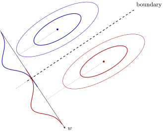
Fisher's linear discriminant (schematic): two Gaussian classes of the same shape (the ellipses are level lines of the densities), and their projections onto the direction , one-dimensional Gaussians that overlap least; the separating line is perpendicular to .
Remark (Fisher's linear discriminant: a historical excursion). In the one-dimensional projection onto the direction vector of the separating hyperplane, the classes are separated in the best way, that is, with the minimum probability of error; the projection axis is perpendicular to the common tangent of the scatter ellipsoids.
This is an interesting picture, a historical excursion: in the early stages of classification theory, people built their algorithms from quite different principles. 1936, Ronald Fisher — the famous Fisher who made the iris dataset. He did indeed work on the linear discriminant that bears his name at that time, but he derived it from completely different considerations; only later did it become clear that it is the Bayes classifier for Gaussian classes. Fisher reasoned as follows: suppose the classes are Gaussian; how do we draw a line such that, when the multivariate Gaussian distributions are projected onto it — a projection onto one axis gives one-dimensional Gaussian distributions — the classes are separated best? One can prove that the perpendicular to this line runs along the tangent between the level lines of the Gaussian densities, and it also gives Fisher's linear discriminant, and it is also the optimal Bayes classifier. That is, there is one more optimality principle here, the best separability of the classes: in the projection they overlap least, and the area of their overlap is exactly what determines the probability of error. It is the same principle of the minimum probability of error. Fisher solved the problem of finding the line onto whose projection multivariate Gaussian densities separate best in 1936 — almost a hundred years ago now.
Fisher R. A. The use of multiple measurements in taxonomic problems, 1936.
Gaussian mixtures with diagonal covariance matrices
One more important special case remains. Let us combine three things: density estimation by a mixture of distributions, the optimal Bayes classifier and, as mixture components, multivariate Gaussians. For simplicity we choose Gaussians with diagonal covariance matrices, in which the features are independent within each mixture component of each class. This is not the naive assumption we had in naive Bayes: there we considered the features independent over the whole space for each class, while here only within one component.
Definition (A Gaussian mixture with diagonal covariance matrices). Assumptions:
- the class likelihood functions can be represented as mixtures of components, ;
- the components have -dimensional Gaussian densities with uncorrelated features: , :
The EM algorithm (numerical features , ):
E-step: for all , :
M-step: for all , , :
Remark: the components are "naive", but the mixture is not "naive".
The notation has become considerably more complicated, but nothing can be done about that: is the class index, the number of the mixture component, the number of the feature. Each class has its own cluster structure, its own mixture of distributions: we could not describe the class by one parametric density, the class is arranged in a more complex way, and we are forced to use a mixture. What should we do? First apply the EM algorithm to estimate the densities — this we already know how to do, there are ready formulas: only now, for each class , in each mixture component , for each feature , we have to compute the mean and the variance by the M-step formulas. I will not write it out further; you just have to sort out all the indices carefully.
Definition (The Bayes classifier on Gaussian mixtures). Substitute the Gaussian mixture into the Bayes classifier:
where are normalising factors; is a weighted Euclidean metric in :
Interpretation: this is a metric classifier in which is the closeness of the object to the -th component of class , and is the closeness of the object to class .
It is interesting to work out what the optimal Bayes classifier will look like. If we write a Gaussian mixture into it, we get an expression that is already painfully familiar to us. A Gaussian distribution with a diagonal covariance matrix is the same thing as a weighted Euclidean metric: a Gaussian is a normalising factor and an exponential, and under the exponential there is a quadratic form, which in the case of a diagonal covariance matrix is written through a weighted Euclidean metric. We measure the distance from the object we want to classify to the centre of the -th component of the -th class, and each feature enters it with its own weight. The density plays the role of a closeness function: it converts distance into closeness — the smaller the distance, the closer to the centre and the larger the density estimate. So we sum the closenesses between the object and the centres of all the components, and if we have accumulated a large total closeness, the object is close to the components of the given class. The total closeness is precisely the value of the mixture of distributions at the given object, that is, an estimate of the degree to which the object belongs to the class .
This whole construction is, on the one hand, the optimal Bayes classifier. And on the other hand — recall, we have already written exactly this formula when we talked about metric classifiers and the method of potential functions, where each class can be described by certain centres, prototypes. We have arrived at the same construction, but now not by a purely heuristic route but through statistical methods: the optimal Bayes classifier, Gaussian densities, estimating these densities by the EM algorithm — this is a much more statistically justified method, but in principle the same one.
The radial basis function network
And we recall it not even for the second time: a very similar construction arises in neural networks too.
Definition (The radial basis function network (RBF)). A three-layer RBF (Radial Basis Functions) network:
The radial basis function network (slide): the first layer computes the closenesses of the object to the centres of the mixture components of each class, the second sums them with weights , the third chooses the class by with the factors .
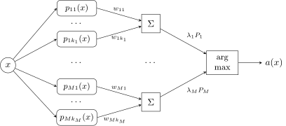
The radial basis function network: the first layer computes the densities of the mixture components of each class, the second mixes them with weights , the third chooses the class by — this is the optimal Bayes classifier.
This is called radial basis functions, or radial basis networks. Look how it turns out: the densities are computed through the distances between the object and certain vectors, the centres , and all these vectors in effect play the role of the weights of a neural network, the strengths of the synaptic connections. The first layer computes the closenesses between the object and certain vectors in the space, the centres of the mixture components of each class. Then we take the closenesses to the components of the first class, the second, and so on, and sum them with the weights that the EM algorithm found for each class; the second layer is in fact an ordinary linear layer of a neural network, averaging the estimates by class. The third layer is : we look at which total closeness estimate, multiplied by as the optimal Bayes classifier requires, turned out to be maximal — it decides the class. Such is this three-layer neural network. One can also recall that a construction of this kind arose in SVM when we introduced kernels.
Remark (The EM algorithm as a method for training radial networks). How the generative RBF-EM differs from the discriminative RBF-SVM:
- the support vectors are not boundary objects of the sample but the centres of local concentrations of the classes;
- a structural description of each class as a set of components, clusters, is built automatically.
Advantages of the EM algorithm: the EM algorithm is easy to make robust to noise; as a rule it converges quite quickly.
Drawbacks of the EM algorithm: it is sensitive to the initial approximation; determining the number of components is a hard problem (simple heuristics may work poorly).
How do radial basis functions built by the EM algorithm differ from those built by SVM? In the EM algorithm we compare the object with the centres of the mixture components of each class, the centres of clusters: each class is some number of clusters, we have described each by its own distribution and measure the distance from the object to the centres of these clusters. In SVM the structure is the same, but the tuning method is completely different: there we compare the object with the support vectors of the classes. A support object is a boundary object; a centre is the centre of a cluster. In SVM we strive to describe the boundary between the classes well, guided by the boundary objects, while here we strive to describe the classes themselves well. Which is better is, generally speaking, debatable. Probably it is still better to describe the boundary between the classes, because, as I said, trying to describe a class's density well everywhere is somewhat excessive for classification. But EM has its advantages: by determining the centres of the clusters in each class, we are not so sensitive to outliers. And SVM has this standard drawback, that it is more sensitive to outliers: an object that has strayed into another class's density will be counted with a very large weight, although it is in essence an outlier.
Conclusions
Bayesian classification models are generative: they model the shape of the classes over the whole space, need a larger amount of data to train, and are less sensitive to noise outliers.
The naive Bayes classifier is based on the assumption that the features are independent.
Three approaches to estimating the density from a sample:
- the parametric approach: Gaussian classes normal discriminant analysis;
- the nonparametric approach: a distance function is given the Parzen window method;
- separating a mixture of distributions: the classes are described by mixtures of Gaussians the RBF network.
The lecture turned out abnormally long, but we learned a lot of interesting things. On Bayesian classification theory: first, a useful formula with which classification models can be constructed from density estimation models. Second, we learned a lot about the naive Bayes classifier. And the three approaches to density estimation — parametric, nonparametric and separating a mixture of distributions — can all be used in the optimal Bayes classifier, and all three lead to constructions, at least two of which we knew before today's lecture: the Parzen window and radial basis functions. We also learned about Fisher's linear discriminant and scolded it: it is old, not very good, and it is better not to use it.
No comments yet
Be the first to share your thoughts.