August 30, 2026 · Lecture · LibreTimes
Machine Learning 1. Lecture 10. Linear Ensembles
Contents
- What this lecture is about
- Ensembles of models
- The formulation of the problem
- Correcting functions
- The problem of diversity of base algorithms
- Simple voting: bagging and random subspaces
- Methods of stochastic ensembling
- Stochastic ensembling in one pseudocode
- The unbiased out-of-bag estimate
- From simple voting to weighted voting
- The random forest
- Weighted voting: AdaBoost
- Boosting for binary classification
- Smooth approximations of the threshold loss function
- The exponential approximation
- The main theorem of boosting
- Convergence
- Classical AdaBoost
- Heuristics and recommendations
- Comparison on model problems
- Why boosting does not overfit
- Experiments
- The theory of generalisation ability
- The distribution of margins
- The drawbacks of AdaBoost
- ComBoost: explicit optimisation of the distribution of margins
- Conclusions
- Seminar
What this lecture is about
Today we have a very important topic, and I will begin straight away with a motivator. The answer to the question "name the three strongest machine learning methods" has stayed the same for more than twenty years: SVM, boosting and neural networks. Clearly everyone talks about neural networks now, but there are many problems where both SVM and boosting are still ahead. And boosting is a linear ensemble, so the topic is important.
A small spoiler. We will begin with general definitions and simple things, and in the second part there will be precisely that boosting with which everything began. It is an old method; something better has been done since, and I will tell about that something in the next lecture. But the meanings here are so dense that one cannot pass them by: it was a very serious turn in machine learning. Not such as with the appearance of large language models, of course, but still. We will talk about that too.
Ensembles of models
What are ensembles about at all? About our solving some machine learning problem, and it turns out to be hard. We build one algorithm, a second, train different models, and somehow nothing works out. Here we have built many different not very successful algorithms, and the question arises: could one successful one be assembled from them?
This suggests an analogy with how we make measurements in physics. If we cannot measure a quantity accurately once, we measure it many times and then average the measurements; the accuracy of the mean grows in proportion to the square root of the number of measurements. On these ideas, in the eighties, people widely put forward the hypothesis that one could probably assemble one strong classifier from many weak ones. That is exactly how Kearns and Valiant formulated this idea in 1989, and that is exactly how it is cited in the foreign literature. Ten years earlier Yurii Ivanovich Zhuravlev formulated it slightly differently and developed his approach, which he called the algebraic approach to pattern recognition. The terminology I will now use comes from the algebraic approach; it is good in that it is very general and covers all variants of compositions altogether.
The formulation of the problem
Let us begin with the formal notation. A training sample is given, and we build base algorithms. An algorithm, let me remind you, is what we call a mapping from to , a trainable mapping. How it is trained is also called an algorithm in Western literature, but in my course, so as not to get confused, I call that a training method.
Definition (The problem of training an ensemble (composition) of models). Given: , the training sample;
- , "weak" trainable base models;
- , algorithmic operators with parameters ;
- , a decision rule of a simple form (without parameters);
- , a convenient space of estimates.
Find: an ensemble
where is a correcting function with parameters .
The criterion for training a "strong" algorithm as an ensemble of base algorithms that are "weak" taken separately:
Yu. I. Zhuravlev. On an algebraic approach to solving recognition or classification problems // Problemy Kibernetiki, 1978 (in Russian). M. Kearns, L. G. Valiant. Cryptographic limitations on learning Boolean formulae and finite automata, 1989.
So the idea is to assemble one good algorithm from many bad ones. For this, in Zhuravlev's terms, such a decomposition of base algorithms is made. Base algorithms are, as a rule, and most classification methods are arranged this way, a superposition. The main mapping translates into some space of estimates ; these are, for example, estimates of the degree of membership of an object in the classes. And then these estimates are coarsened and turn into : in a classification problem is a discrete set. If we tried to do the correction, the aggregation, over the answers of the base algorithms themselves in the discrete set , nothing much would come of it: it would be a rather weak construction. For correction we need finer estimates: they contain more information about the classes.
So a decomposition arises: a superposition of two, in the general case trainable, transformations and . The are called algorithmic operators, the decision rule. Now we, as it were, break the base algorithms, tear away from , and say that we will carry out the composition, or correction, or aggregation of the base algorithms in the space of estimates . This is done by a correcting operation, a function from to : at the input it takes answers of the base algorithmic operators and aggregates them somehow into the answer of the composition. This is to a large extent a technical device of decomposition; it allows us to work in convenient spaces of estimates and to introduce them as we like.
Example (Spaces of estimates and decision rules).
- Classification, a finite set; , : no decision rule is used.
- Binary classification, :
, is a real-valued classifier, . 3. Classification into classes, :
, , . 4. Regression, ; : no decision rule is used.
Let me explain on examples what a space of estimates is and how decision rules can be arranged in this connection. The first example is classification. One can, in principle, make a composition over the classifications themselves; then is the identity transformation, the decision rule is simply not used, and is the space of classes itself. Why it is bad to do so I have already said: in the space the class of correcting operations is too poor; there is nothing to choose from except perhaps some voting.
The second example is classification into two classes; we have already seen many such problems. The classes are denoted and , and the algorithm is arranged as a superposition of the decision rule and the base algorithmic operator , in Zhuravlev's terms. In the English terminology that has taken root, is called a real-valued classifier. The decision rule here is simple and untrainable: it is simply the sign function, there are no parameters in it.
The third example: what if there are many classes? We have seen this construction, for example, when we talked about metric classifiers or about logistic regression, and will see it again when we talk about Bayesian classification theory. The classifiers are arranged as an over the classes, and is the estimate of the degree of membership of the object in the class . These are our base algorithmic operators, or real-valued classifier, but now it returns not one number but as many numbers as there are classes: for each class its own estimate of the degree of membership. And the is the decision rule, now of arguments.
And the fourth example, similar to the first: in regression problems decision rules need not be used, because is a space convenient in itself for building any correcting operation in it.
Correcting functions
Now about aggregating, or correcting, functions; I keep saying both these words, because in the literature they are called both ways.
Definition (Correcting (aggregating) functions). General requirements on the aggregating function :
- , a Cauchy mean, ;
- is monotonically non-decreasing in all .
Examples of aggregating functions:
- simple voting:
- weighted voting:
- a mixture of experts with competence functions (gating functions) :
Let us think about what axiomatic requirements should be imposed on an aggregating function. Probably the range of its values on the answers of the base algorithms should lie between the minimal and the maximal of them: it would be strange if we went outside this range; there we no longer have information about how the base algorithms worked. Any such aggregating value in this range is called a generalised Cauchy mean: these are some variants of averaging, but there can be many different ones.
The second requirement is more substantial: must be a monotone function in all its arguments . Imagine this situation: all the base algorithms return on an object the same answer as before, and one of them begins to return a larger one. It would be strange if as a result of the correction the answer of the composition decreased. This is a very natural consideration, and this requirement is directly the definition of a monotone function of arguments.
What aggregating functions are most often used in practice? Averaging, of course; I began with that: the mean of physical measurements is more accurate than an individual measurement. Simple averaging in the case of classification is called simple voting; it is probably the simplest thing one can think of. In weighted voting we add the coefficients ; before, they were all the same. Some base algorithms work better, some worse; those that are better we trust more, and they should probably be given a larger weight. So is in essence a discrete distribution on the weights: non-negative coefficients normalised to one.
And the coolest generalisation of the mean is a mean in which the coefficients are replaced by functions of . We say: in one part of the space one base algorithm works well, and in another another; and these parts of the space are described by the competence functions of the base algorithms, or gates. In English these are gating functions; in Russian they are translated in different ways, as sluices, as valves. Today we will talk about simple and weighted voting, and we will touch on mixtures of algorithms next time.
The problem of diversity of base algorithms
Let us return once more to the analogy with physical measurements. Why will it not work directly in machine learning problems, and how can this idea still be advanced?
Definition (The problem of diversity of base algorithms). Measuring a random variable from independent observations :
- , the expectation of the mean;
- , the variance as .
But the base algorithms are not independent random variables:
- they solve one and the same problem;
- they are tuned to one target vector ;
- they are usually chosen from one and the same model.
Ways of increasing the diversity of base algorithms:
- training on different (random) subsamples;
- training on different (random) sets of features;
- training from different parametric models;
- training with the use of randomisation;
- (sometimes even) training on noisy data.
The analogy works well when the observations are independent: then we know that with the mean we estimate the expectation, and the variance of this estimate tends to zero as tends to infinity. But the base algorithms, or rather their answers, the vector of answers, are certainly not independent random variables. Why? Because the base algorithms solved one and the same problem, we trained them on the same data, on one and the same target vector, and, moreover, they are usually also chosen from one and the same model. There are, of course, approaches where heterogeneous classifiers are aggregated: let us take a neural network, a decision tree, something else like nearest neighbour, models that in themselves divide the space differently. Such an approach exists, but it is rarely used; most often the base algorithms are taken from one model.
So the variance will certainly no longer decrease at the same rate as when averaging independent variables. But such an aim is still set: one still wants to achieve a decrease of the variance with the growth of the number of base algorithms. What should one strive for to achieve this? That the base algorithms be different: if they are the same or almost the same, there will be no sense in building a composition from them.
Here there is a contradiction, a double-edged sword. On the one hand, the base algorithms must work reasonably well, at least better than random guessing, for a good solution to be assembled from them. On the other hand, if they all work well, it means they are similar to each other and lack diversity, and then there is no sense in building a composition. Diversity will help reduce the variance: the base algorithms will not, of course, become independent variables, but they will depend on each other less, and this will probably have a positive effect on the variance decreasing as the number of base algorithms grows.
How can diversity be increased, what ideas come to mind here? One can train the base algorithms not on the whole sample, one and the same for all, but on random subsamples: we introduce some noise, randomness, but all the base algorithms still solve one and the same problem; we only shorten their training samples. One can cut down their sets of features: random subspaces of features. One can, as I have already said, take them from different parametric models. One can deliberately introduce some randomisation. One can even deliberately spoil the data, put noise either on or on ; this too is done, and it even works. Let us try to combine at least some of these ideas and do it in the simplest way possible.
Simple voting: bagging and random subspaces
We have gone through the setting-up stage, given definitions, and now we will take up methods. The first method is called bagging. This word was cooked up from bootstrap aggregating.
Methods of stochastic ensembling
Definition (Methods of stochastic ensembling). Ways of increasing diversity by randomisation:
- bagging (bootstrap aggregating): subsamples of the training sample "with replacement"; each sample gets
of the objects as ;
- pasting: random training subsamples;
- random subspaces: random subsets of features;
- random patches: random subsets of both objects and features;
- cross-validated committee: the sample is split into blocks (-fold) and trainings without one block are done.
Let be a method of training on a subsample that uses only features from :
is empirical risk minimisation.
Leo Breiman. Bagging predictors // Machine Learning, 1996. Tin Kam Ho. The random subspace method for constructing decision forests, 1998.
The bootstrap is choosing objects "with replacement": we choose a random object from the sample but return it, so that we have a chance to choose it again, perhaps even several times. With such choosing with replacement not all objects get into the sample: some will be chosen several times, and some not once. We keep the sample size the same, : choosing objects with replacement, we get exactly as many objects as there were, but this sample will be, as it were, a random incarnation of the original one; there will be repetitions in it. What is the share of objects that will enter the bootstrap sample? It is estimated very well, and as tends to infinity we will see here literally the definition of the number : it is . That is, roughly two thirds of the sample get into the subsample each time, and there will be repetitions among these selected objects.
This is not the only way, though the most popular. Why? Because many interesting theorems have been proved about the bootstrap, including that this sample is unbiased. Do not be troubled that objects repeat in it, although there were no repetitions in the original sample, and that something seems wrong with such a distribution. Nevertheless it is a sample from the same distribution, and in this sense it is unbiased. The bootstrap has useful theoretical properties, so it is often used.
But, of course, one can also use simply random training subsamples: pasting. Especially when you know that in your particular problem the training sample is highly redundant: you have, perhaps, a million objects, and you suspect that you will tune the model quite well on a thousand. Should one sample a million again from a million by bootstrap? By and large, no: one can randomly reduce the amount of data and, if the data were originally redundant, not lose much in quality.
What else can be done? Let us look at the "objects–features" matrix: the rows are objects, the columns features. We have just chosen a random subset of rows; the same can be done with the columns. These are random subspaces: we choose a random subset of features. And if we pull out of the "objects–features" matrix a submatrix, a subset of rows and a subset of columns, these are random patches on the matrix. And finally, one can do all sorts of cross-validations: split the sample into blocks and train on all the blocks except one. There are in fact many different techniques, and the essence of all of them is one: select a random part of the data on which one can nevertheless train a decent model.
Now let us agree: we have a training method , which takes as input a subsample of objects and a subset of features from the set of all features. We will never get inside the training method, and this is really great. This is called a wrapper over an already existing training method: we simply feed it a subset of the data at the input.
Remark (Why choose with replacement). Choosing with repetitions is done in order to preserve unbiasedness. I would say that this is a kind of idée fixe that came from statistics: unbiasedness really is guaranteed, it is a simple and clear technique, but there is no sense in doing exactly so. One can make random subsamples too, and everything depends strongly on how redundant the data in the problem are. If you have a million objects, and a thousand is just about enough to build a model, then there is no reason to do a bootstrap either of a million objects or of a thousand: if you randomly choose a thousand out of a million, repetitions will not arise anyway. Do sampling without replacement.
Remark (Stratification). Statisticians and sociologists are constantly fussing over a representative sample; are there ways to make subsamples that preserve the properties of the original one? There is a technique used very often in machine learning: stratification of the sample. For example, when we divide the data into train and test and want the share of objects of different classes in them to be the same. It is done very simply: we set a proportion, how many objects go into train and how many into test, for example , and in this proportion we randomly divide each class separately into two parts. Then the train parts of all classes are combined, and the test parts too. In this way we guarantee that the representation of objects of all classes in train and in test is the same.
This is especially important in problems with imbalanced classes, when there is very little of one class, or a hundred times less than of another: a random subsample may lead to the small class entering, for example, the test sample with literally a few objects, or not entering at all. Roughly the same can be done in bagging or in the bootstrap: ensuring by construction the same proportions of data of different classes.
This story has a mass of continuations. Over features too, generally speaking, stratification should be done, but that is a much more complicated story: if some feature contains rare but anomalous observations, they should be distributed evenly between train and test. It is the same kind of problem as with imbalanced classes, only now over a feature. I do not go into the details, but remember the word "stratification": it is a very useful and correct thing.
Stratification has no minuses. It does not make the model memorise rare objects: after all, we want train and test, although they are different and random, to have the same statistical properties, to be from the same distribution. We want, on the one hand, to make a random split, and on the other, for the subsample to be representative, to have the same properties as the general population. If the amount of data is insufficient, this property may by chance be critically violated, especially with class imbalance or when the data are a mixture of distributions, one of which is plentiful and another scarce: representatives of the small class may disappear altogether from some subsamples in the split. This is like cohort studies in sociology, where one strives for all strata of society to be represented in the sample. But there it is the organisation of surveys and data collection, while for us it is, as a rule, a split into train and test or bagging for a composition.
Stochastic ensembling in one pseudocode
Definition (Methods of stochastic ensembling in one pseudocode). Input: the training sample ; parameters: ;
- , the size of the training subsamples;
- , the dimension of the feature subspaces;
- , the threshold of quality of base algorithms on training;
- , the threshold of quality of base algorithms on validation.
Output: base algorithms , .
- for all :
- a random subsample of size from ;
- a random subset of cardinality from ;
- ;
- if , do not include in the ensemble;
- if , do not include in the ensemble.
The ensemble is simple voting:
In this pseudocode I have combined two methods. Bagging is based on bootstrap aggregating, on forming training subsamples by bootstrap, and the random subspace method on choosing random subsets of features. One can do either the one or the other, or both at once.
What happens here? In turn, for all base algorithms, we take a random subsample, and there may be many methods of choosing a random subsample, I have just roughly described them; the pseudocode does not fix the method. We have formed a random subsample and a random subset of features, and we build a base algorithm. It may happen that the subsample is too small or there has simply been a failure, and the base algorithm has come out bad. Let us introduce a parameter that controls the quality on the training subsample itself: if the error is above the given threshold , we will not include such a base algorithm in the ensemble; it did not come out. For example, we look, and its share of errors on training is more than a half. Why can this happen? Some needed features did not enter; there were not enough informative features to build a classifier of acceptable quality. Let us not take it, let us discard it at once: it was unlucky.
And if we have random subsamples being formed, then there are objects left on which we did not train. That is great! It means we can get an unbiased estimate of the generalisation ability of the base algorithm, and put a threshold on it too, : if the base algorithm has come out too bad already from the point of view of working on an independent validation sample, we will not take it into the ensemble either. Such is the method, please welcome it: bagging, even with a generalisation towards the random subspace method.
And what to do with these base algorithms? The simplest answer there can be: simple voting, just average them. We tried to make them as independent of each other as possible. And by the way, we built them on random subsamples, without peeking at each other, which means that the loop over can be executed in parallel altogether. This is very good news: the method is very easily parallelised; the base algorithms can be built independently of each other.
The unbiased out-of-bag estimate
One more very important thing we get here for free when we build base algorithms on random subsamples. is a random subsample, and then turns out to be a test sample: there are objects on which we did not train this base algorithm, and it would be good to check it on them along the way. How is this to be done?
Definition (An unbiased estimate of errors). Out-of-bag is an unbiased estimate of the ensemble on an object:
An unbiased estimate of the error of the ensemble on the training sample:
where is the value of the loss function on the object .
Estimating the importance of the features , :
where, when computing for , the values of the feature are randomly shuffled on all objects .
Look what an unusual idea. For each -th object let us take the set of base algorithms that did not train on it. Recall bagging: each base algorithm trains on roughly of the objects, so roughly of the base algorithms did not train on each given object. That is quite a lot: if we build a composition of a hundred base algorithms, roughly 37 of them, give or take, did not train on a given object. We can average over them, precisely over these algorithms, not over all, but only over those for which the -th object was a validation one and not a training one.
Now we average these out-of-bag estimates over all objects and look at the mean losses over the whole sample. This will be an unbiased estimate of the error of the ensemble on the training sample. This is really great: without explicitly doing a hold-out split into train and test, we have got a split into train and test for each base algorithm of its own, and have been able to use all these splits at once to estimate the generalisation ability of the whole ensemble.
What does this allow? Well, simply making an unbiased estimate of quality is already great. But one can also extract from it estimates of the importance of features. Since the out-of-bag estimate is unbiased, we can apply it to an ensemble in which the -th feature is used and to an ensemble from which the -th feature has been removed. One can do this honestly: when training the base algorithms, forbid them all to use the -th feature. One can, but it takes long. Or one can do it more simply: when computing for out-of-bag, we take and randomly shuffle the values of the feature on all validation objects. We will not rebuild the model; let it still use this feature, but on the validation objects we shuffle its values among the objects. What have we done? We still feed the model this feature from the same distribution at the input, only it is shuffled: it has become noise, uninformative. If the out-of-bag sagged badly as a result, it means the feature was very important for the model. The greater the relative difference in the quality of the model with the spoiled feature and with all features, the higher the informativeness of the -th feature. This estimate is built into all decent implementations of bagging, and the estimates of the informativeness of features are, as a rule, built in too. They can and should be used.
From simple voting to weighted voting
To finish with simple voting: can one, having built base algorithms as we have just done, use not simple voting but weighted voting?
Definition (Converting simple voting into weighted voting). A linear model over ready features :
Training: least squares for regression, logistic regression for classification:
Regularisation: or LASSO: .
The naive Bayes classifier assumes the independence of the random variables and gives an analytical solution:
where is the estimate of the probability of error of the base algorithm .
Yes, of course one can: then you simply build a linear classifier over the base algorithms as over features. You have already trained them; for you they are fixed functions on the objects of the sample, and now one can build a linear classifier over them as over features, and if it is a matter of regression, a linear regression. If uninformative ones have to be found among these base algorithm features, please: we use LASSO, impose constraints on the coefficients , or inequality constraints, so that there are no negative ones among them. These ways in effect allow the composition of base algorithms to be regularised and the superfluous ones thrown out of it, if there are any.
There is one more way; we will understand it better when we have the lecture on Bayesian classification theory and learn what the naive Bayes classifier is. It assumes that the features are independent; in our case, building weighted voting, we will assume the independence of the base algorithms. Now, stop, stop, stop: we only just said, ten minutes ago, that this certainly does not hold, and even in bagging we try to make the base algorithms as different as possible. Well, still, then as a heuristic. If the base algorithms are independent as random variables, the optimal solution for the coefficients can be obtained analytically, and it looks like this, where is the share of errors, the estimate of the probability of error of the base algorithm. Clearly: the more a base algorithm errs, the smaller its will be, and if it errs fifty-fifty, that is, is engaged in random guessing, then will be zero. By such formulas, without any optimisation, without any training, fairly crudely, but already taking into account the quality of the individual base algorithms, one can compute the coefficients .
The random forest
How did things develop further? Bagging was invented around 1996, as far as I remember, and people at once began to try different base algorithms, to try to answer the question over which family of base algorithms this aggregation technique works better. They tried a lot: neural networks, SVM, nearest neighbours, rules, and decision trees, and settled on decision trees. Why? Because they have one remarkable drawback that bagging turns into a merit. Decision trees are very unstable to changes in the composition of the sample: if you change even something small in the sample, and all the more when you do bagging and train on random subsamples, the trees become highly diverse, and their quality may suffer. But that is exactly what is needed for aggregation! When building individual trees, instability, a strong dependence of the structure of the tree on the composition of the training sample, is a drawback; we always say that it is bad. But in this case it is, on the contrary, good, because it increases the difference between the base algorithms.
Definition (The random forest (Random Forest)). Rough training of trees for a random forest:
- bagging over decision trees, without pruning;
- the feature at each node of a tree is chosen from a random subset of of the features.
By default for regression, for classification.
Parameters that can be tuned (in particular, by OOB):
- the number of trees;
- the number of randomly chosen features;
- the maximal depth of the trees;
- the minimal number of objects in a subsample being split;
- the minimal number of objects in the leaves;
- the criterion for splitting the internal nodes of a tree.
Breiman L. Random Forests // Machine Learning, 2001.
This is what the Random Forest method consists of: we do bagging over decision trees, and we do not try to make the individual decision trees as good as possible. In particular, we do no pruning, and the feature at each node is chosen from a random subset of features. We do still keep an element of training, an element of optimisation. Remember, in a decision tree, when choosing the branching criterion at each node, we go over all the features, simply a loop over from one to ? Well, here the search is not over all the features but over a random subset of of the .
How to take this number is the subject of a certain holy war. Clearly it depends on the problem, on the number of noisy, noise, uninformative features; it is an individual property of each problem, and there are no universal recipes here. In Leo Breiman's paper there was this recommendation: roughly a third of the features for regression and, for some reason, the root of for classification. I would say that it depends rather on the problem after all, and one should search, not use heuristics of this sort.
In random forests there are not many parameters, and by choosing them one can build a very effective ensemble. There will be many trees, each individual tree will work poorly, but all together, even after simple, unweighted voting, they give a more or less reliable classifier. Random Forest is considered one of the best universal machine learning methods: it cracks problems of any complexity. If the boundaries between your classes are of very complex shape, Random Forest is what should be applied.
What can be tuned here? Clearly, the number of base algorithms, of trees. The number , how many features we select at random; this is a very important parameter, which is, as a rule, chosen, and literally a few values are enough to search over. The maximal depth of the trees: if the depth is small, many trees will be needed, and individually they will not be very good; the greater the depth, the better the quality of the individual trees, but they may turn out overfitted. One can search over much else too: the minimal number of objects of the sample from which we determine the feature in the branching criterion; the minimal number of objects falling into a leaf, which is something like a pre-pruning criterion. People also tried different branching criteria. But the main parameters are, of course, the first three.
On the internet there is a huge number of examples of what compositions of decision trees look like when enough trees are built. On the slide are wonderful pictures from Alexander Dyakonov's blog, where there are many articles about machine learning, including about ensembles: the separation of a sample by individual trees (with their bootstrap subsamples) and by a random forest of 10, 100 and 1000 trees. The sample is the famous "two bananas", or two moons: classes penetrating each other, a hard problem for a linear classifier. For trees it is not very simple either: one can see that an individual tree classifies not very well somehow; the separating surface of individual trees is angular. But look how everything is smoothed out: even ten trees are, by and large, enough for the boundary to be built more or less, and with a thousand trees it did not particularly improve. When angular trees are averaged, even ten turn out to be enough for the separating surface between the classes to be smoothed out.
On the topic of decision forests, from the mid-nineties and especially from the early 2000s, there was a huge amount of research, and people tried to build all sorts of things here. I will not dwell on this; well, for example, rotation forest. It turned out that if we build trees like this, not very accurately, on subsets of features, and then allow ourselves to optimise the rotation of the whole tree in space, then optimising these rotations, even roughly, allows a classifier to be built that works even better. Not always, without a guarantee, but still it is one of the successful heuristics.
Remark (Rotation forest and oblique trees). Imagine that in the space of two features you have built a tree and its separating surface. It is angular, and all its lines are parallel to the coordinate axes, because the nodes of the tree use threshold conditions on individual features; in the last lecture we saw what a tree looks like on Fisher's irises. In rotation forest we take an already built tree and rotate it as a whole in the space of the features over which it was built. This seems strange, not grounded in any way, but for some reason it works: a rather unexpected heuristic that turned out to be successful in some problems. In the next lecture there will be a picture where one can see how rotation forest smooths out the separating surface as the number of base algorithms grows: there are many of them, and each is rotated by its own angle.
Do not confuse this with oblique decision trees, in whose nodes one can choose linear combinations of features: not simply go over features and a threshold for a feature, but in essence build a linear classifier at each internal node of the tree. That is a different idea: in rotation forest an already built tree is rotated as a whole.
Advantages:
- a wrapper (envelope) method over the base training method;
- suitable for classification, regression and other problems;
- simple implementation and simple parallelisation;
- the possibility of obtaining unbiased OOB estimates;
- the possibility of estimating the importance of features;
- RF is one of the best universal methods in ML.
Limitations:
- veeeeery many base algorithms are required;
- stable base training methods are hard to aggregate.
So what are the advantages and limitations? The advantage is that this is a wrapper method: the base algorithms can be anything, we simply feed them a subset of objects and a subset of features at the input and do not get inside. This is a splendid property: methods of this kind are easily generalised to regression, classification and other machine learning problems; everything depends on how the loss function is set, and in different problems it is set differently. A very simple implementation, very easily parallelised: bagging is good precisely for this purely technical feature. There is the unbiased out-of-bag estimate of quality and the possibility of estimating the importance of features from these unbiased estimates. And, as I have already said, Random Forest is generally one of the leaders in universality: the hardest problems from the most diverse fields are solved by the Random Forest method, and, as a rule, a rather high generalisation ability results. Thanks to what, we will still talk about today, but in rough terms: thanks to the base algorithms being averaged and their errors compensating each other: the error is smeared out, its variance decreases.
But there are also limitations, drawbacks. First, sometimes very many base algorithms are required; these may be not even hundreds but thousands. And if we are talking about decision trees, what do we love them for? For being interpretable; they have a very simple and clear structure. But if we take a thousand trees, there is no longer any question of interpretation; interpretability is lost. And one more limitation, which, if we have time, we will work on at the end of the lecture. Trees are unstable; they respond strongly to the composition of the training sample and even change their structure. But there are methods that are, on the contrary, super-stable, for example SVM. Building bagging from SVM is something nobody has particularly managed, by and large, precisely for this reason: you make subsamples, and the set of support objects stays the same or almost the same, and no diversity of base algorithms results.
Weighted voting: AdaBoost
Now the most interesting and the most important thing for today's lecture: boosting, as it was invented in the mid-nineties. I will tell about AdaBoost, with which all this hype began.
Boosting for binary classification
Definition (Boosting for the binary classification problem). Given: , , , ; means abstaining from classification (in particular, the may be logical rules).
Find an ensemble with weighted voting:
Criterion: the minimum of the number of errors of the ensemble on training:
The two main heuristics of boosting:
- fixing when adding ;
- a smooth approximation of the threshold loss function .
We consider the problem of classification into two classes. The base algorithms return , or ; zero means abstaining from classification. Clearly, when we average by weighted voting, a zero answer of a base algorithm means that in the composition it is not taken into account on this object. In English this property is called abstain: classification algorithms are supposed to return plus or minus one, but if they return zeros, they are said to abstain from classification. Here a simplification is used that I scolded at the beginning of the lecture: we do not apply the decision rule to the base algorithms; they themselves already give discrete-valued answers, and we average these answers, and take the sign only of the composition. This is a limitation that we will later give up: in the next lecture I will tell about gradient boosting, which removes this limitation completely and passes into AdaBoost as a special case.
So weighted voting is a linear classifier where the base algorithms are used as features; is the number of base algorithms. Our task is to build a composition, that is, to find at once all the base algorithms and the coefficients at them so as to minimise the number of errors on the training sample. The difficulty is that the problem comes out heterogeneous. If it is posed as simultaneous training of both and for all base algorithms, it stops being a wrapper, while we would dream of making a method that uses standard methods of training base algorithms.
For this the following heuristic is introduced: we will add base algorithms to the composition one at a time, considering that all the previous ones have already been built and fixed. That is, this is a greedy method of building a composition. And one more heuristic: we will use smooth approximations of the threshold loss function. The loss function here is in effect "the margin is less than zero", an unpleasant, piecewise-constant one, and we will replace it by a smooth loss function. We have already met this trick: logistic regression, SVM and much else. The only question is which approximation we will take.
Smooth approximations of the threshold loss function
The threshold loss function (red) and its smooth approximations as functions of the margin (slide): , exponential; , logarithmic; , quadratic; , Gaussian; , sigmoid; , piecewise-linear. They all pass through the point .
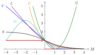
The threshold loss function (red) and its smooth approximations as functions of the margin : , exponential; , logarithmic; , quadratic; , Gaussian (here , ); , sigmoid; , piecewise-linear. They all pass through the point .
| Loss function | Method | |
|---|---|---|
| exponential | AdaBoost | |
| logarithmic | LogitBoost | |
| quadratic | GentleBoost | |
| Gaussian | BrownBoost | |
| sigmoid | ||
| piecewise-linear | from SVM |
In the boosting I will now tell about, the approximation is exponential. It was tried first, and this gave a semi-analytical solution of the optimisation problem, which is splendid and very convenient. Then people began to try all the others too, got, of course, to logistic regression and to SVM, and different variants of boosting over other loss functions appeared. Each such study was a separate scientific paper finding out whether it works better than AdaBoost or worse. But historically the first in this line was AdaBoost, so that is what we will now consider.
Remark (What the right branch of the parabola is for). I am showing this picture not for the first time; today there is one more occasion. There is the threshold loss function, and it can be replaced by a continuous or smooth one, and depending on this replacement a huge number of different methods appears. Moreover, historically each of them could arise from its own considerations: logistic regression is statistics, SVM is geometry, and BrownBoost with the Gaussian curve appeared from modelling Brownian motion; I will not tell it in detail, one can look at the paper. But in rough terms it is clear what it does: it drives the weights of anomalous outliers to zero so as not to train on them. AdaBoost with an additional heuristic, let us detect the objects whose weights have grown anomalously and simply discard them, does the same; BrownBoost is a more theoretically grounded heuristic. In general the family of smooth or continuous approximations of the threshold loss function is infinite, and they do not even have to pass strictly above the threshold function.
And here is the parabola. One asks: what is its right branch doing here, why penalise large positive margins, why not throw it away? In fact there is such a loss function too, it is just hard to draw it here: the left branch as in the parabola, and zero for margins greater than one. It is the same positive cut-off as in the SVM loss function, the piecewise-linear hinge loss, only instead of the sloping linear segment it has a piece of the left branch of the parabola: we took the SVM loss function and squared it. This can be done; it will deprive us of support objects and other delights of SVM, but in principle one can work this way. And what is the right branch kept for? There is such a method, Fisher's linear discriminant; we will get to it when we talk about Bayesian classification theory. There such a loss function arises because we try to describe each class by a Gaussian distribution. There is, generally speaking, no sense in this: we try to describe the distribution of objects in those regions of space that are far from the separating surface, and penalise them for not being described by a multivariate Gaussian distribution. This is rather silly, outdated and does not work very well in practice, but as a fact, there are such loss functions too.
The exponential approximation
Definition (The exponential approximation of the threshold loss function). An upper bound of the quality functional :
The normalised weights: , .
The weighted share of wrong (negative) and correct (positive) classifications with the normalised weights :
is the weighted share of abstentions from classification.
Y. Freund, R. E. Schapire. A decision-theoretic generalization of on-line learning and an application to boosting, 1995.
So what do we do? We build an upper bound of the quality functional : we replace the threshold function "the margin is less than zero" by the exponential function and get an upper bound for our functional, which will be denoted . Now let us use a remarkable property of the exponential: the exponential of a sum equals the product of exponentials. We agreed that all the previous base algorithms have already been built and are fixed for us, so we take their sum under the exponential out, and it will be a factor, and the second factor, a separate exponential, will be the algorithm we are now going to build, and the coefficient at it.
Let us think about what the first factor, the weight , means: which objects will get large weights and which small ones? By and large it is clear: if the margin is large and negative, the exponential will be large. This means that if on the -th object the whole previous composition made a big error, then for building the next algorithm precisely this object will have the largest weight. Large weights go to those objects on which the whole previous composition erred most. This seems very logical, and we understood it literally at once, after the very first line of the derivation, when we passed to the exponential approximation of the threshold loss function.
We will normalise the weights and denote the normalised weights . Next we will need a definition that will be used in the theorem. For an arbitrary normalised non-negative weight vector , it is the same as , but for generality I write , let us define the weighted share of wrong classifications : it is a sum over objects with weights whose sum equals one, and the condition in brackets means that the algorithm errs on the object, errs but does not abstain from classification. In exactly the same way, the weighted share of correct classifications , where the condition in brackets means that the base algorithm gives the correct answer on . One can also compute the share of objects on which the base algorithm returns zero, that is, abstains from classification: it equals . A base algorithm has three possible answers, plus or minus one and zero, and the shares will of course sum to one, because the weights are normalised.
The main theorem of boosting
Classical AdaBoost was invented for the situation where the base algorithms do not abstain from classification. A little later the same authors, Freund and Schapire, invented a scheme with the abstain property, abstention from classification, and showed on experimental data that such compositions work better. That is, if a base algorithm is not confident in its answer, let it rather return zero: let it not lie but honestly say that this is not its area of competence. For the composition this turned out to be good, so I begin at once with this generalisation, although it was invented a year later.
Theorem (The main theorem of boosting (Freund, Schapire, 1996)). Suppose that for any normalised weight vector there exists an algorithm that classifies the sample at least slightly better than at random: . Then the minimum of the functional is attained at
R. E. Schapire, Y. Singer. Improved boosting algorithms using confidence-rated predictions, 1999.
Suppose that for any normalised weight vector, in the base family of algorithms, the parametric family of functions from which we choose , there exists an algorithm that classifies the sample at least slightly better than at random. The requirement is non-trivial, because it contains the quantifier "for any normalised weight vector". If one takes a fixed weight vector, practically any family will satisfy this requirement. But "for any" is already a stronger restriction. In practice, however, as a rule all the families we use, decision trees certainly, satisfy this requirement, so it does not restrict us much.
Then the minimum of the approximated functional is attained when two very interesting formulas hold, which in effect tell us that base algorithms can be built very easily and quickly, and the coefficients at them determined simply by an analytical formula. The theorem says that one has to maximise this interesting criterion: . When in the last lecture we talked about informativeness criteria for logical rules, I wrote out this criterion and promised to show where it comes from. Now there will be the proof of the theorem, and you will understand that it comes from the exponential approximation of the threshold loss function. And for there is this simple formula.
The proof is not difficult, very instructive and beautiful, and I hope we will understand it quickly. This is the rare case when I do insert a mathematical proof into my course: it seems to me interesting.
Proof. Step 1. The first, very simple observation: for any real and any taking the discrete values , the identity holds
We simply expanded the exponential over the possible values of ; the identity is completely trivial, but we will need it now. Let us set for brevity and . The weights we have already computed at the previous iterations; for us they are simply numbers. Let us substitute the identity into the exponential , expand it into three terms and distribute them into three sums:
and are common factors that come out of the sums, and the sums themselves are the quantities we have just introduced: the weighted share of correct answers, the weighted share of errors and the weighted share of abstentions from classification. I have normalised the weights, that is, divided by the sum of all weights; having divided, one has to multiply, so the factor arises. And this is nothing other than . Why? In each is multiplied by an exponential that depends on the current base algorithm, while all the previous such exponentials over all the previous base algorithms have multiplied together and given the weights ; so is simply the sum of the . Shortening the notation, we get
This is a function of , and one can see that enters only these exponentials and nowhere else, and a function of the base algorithm , on which and depend. Look what possibility we have now: to solve the problem in analytically. First let us minimise over ; we differentiate:
We have got what was required: ; we have proved half of the theorem. The coefficient came out through the logarithm because the approximation of the threshold loss function was exponential, and only because of that.
Step 2. Let us substitute the optimal value back into . Everything will simplify, and we will recognise the formula of the square of a difference:
Since does not depend on and , minimising is equivalent to maximising the square of the difference. It can be maximised in two ways: either with , or with ; but the second case is excluded by the condition of the theorem, by which the base algorithm can always be chosen so that is greater than . So we drop the absolute value and get the criterion from the statement of the theorem: . The theorem is proved.
Freund and Schapire are geniuses, of course: to think of such a simple thing and to prove so simply and elegantly that with the exponential approximation of the loss function compositions are easily built by an iterative process, where each base algorithm is built by the criterion of maximum of . Great!
Convergence
Let us obtain a couple more facts as corollaries. The first: it turns out that we have convergence on the training sample; in the limit we get an algorithm that makes no errors at all. Whether this is good or bad has to be discussed separately. It would seem that it is bad, because it is guaranteed overfitting; but it is good if we are talking about the ability of the classifier to minimise the number of errors on training.
Corollary (Convergence). If at each step the family and the training method ensure the building of a base algorithm such that
for some , then in a finite number of steps an algorithm will be built that makes no errors on .
That is, if the family is so rich that at each step it ensures the building of a base algorithm whose is not simply greater than zero but greater than some positive number , then in a finite number of steps a correct algorithm will be built, making not a single error on the training sample. The proof is simple and beautiful.
Proof. converges to zero at the rate of a geometric progression. Let us bound from above: first, , and in the course of proving the theorem we saw that is the product of and :
At each step of boosting, at each passage from to , the current estimate is multiplied by a number less than . If , a moment will come when . But is an upper bound for , and is by definition a sum over the objects of the sample, taking discrete values: . If at some iteration it has become less than one, it has nowhere to go: , zero errors on the training sample.
This is an interesting fact about convergence, but it is, of course, convergence not in the sense of generalisation ability but only in the sense of the number of errors on the training sample.
Classical AdaBoost
One more corollary. As I have already said, the original variant of AdaBoost was invented for base algorithms that cannot abstain from classification. Then it is simply a corollary of the previous theorem.
Corollary (Classical AdaBoost (Freund, Schapire, 1995)). Let there be no abstentions, ; then . Suppose that for any normalised weight vector there exists an algorithm that classifies the sample at least slightly better than at random: . Then the minimum of the functional is attained at
Y. Freund, R. E. Schapire. A decision-theoretic generalization of on-line learning and an application to boosting, 1995.
The share of correct answers we can express as , simplify the criterion for building base algorithms and see that it has become the ordinary formula of the method of empirical risk minimisation, only with weighted objects. is the weighted share of errors on the training sample: our usual functional, a sum over all the objects of the sample of the binary loss function "error or not error", but each object is taken with its own weight . A huge number of machine learning methods are very easily adapted to empirical risk minimisation with weighted objects: adding weights to the optimisation problem and adapting the optimisation method to such a formulation is a simple exercise; it is always easy to do.
So such a method, AdaBoost, adaptive boosting, adaptive because it adapts the composition by adding each base algorithm so that it corrects the errors of the previous ones, also turns out to be a wrapper. If you can tune base algorithms on a weighted training sample, you can easily use AdaBoost to make a composition.
Definition (The AdaBoost algorithm (in the original variant)). Input: the training sample ; the parameter .
Output: the base algorithms and their weights , .
- initialise the weights of the objects: , ;
- for all :
- train a base algorithm: ;
- ;
- update the weights of the objects: , ;
- normalise the weights of the objects: ; , .
Let us put everything together. Two main operations: we train a base algorithm as usual, but with weights on the objects of the training sample, and determine the coefficient by the formula from the theorem. The weights of the objects need not be recomputed from scratch each time: as the theorem shows, and we understood it even before the proof, after each base algorithm is built the weights are simply multiplied by these exponentials. True, after multiplication they have to be normalised.
When AdaBoost appeared, the whole machine learning community rushed to do experiments with boosting and, unexpectedly for itself, discovered an interesting thing: boosting does not overfit, although the number of base algorithms grows. It had always been considered that the complexity of a model is a misfortune that one has to get away from somehow; complexity has to be limited somehow. But here it turns out that the complexity of the composition can be increased practically without limit, that is, the number of base algorithms increased, and the generalisation ability gets better and better: the more base algorithms, the better the composition works. Intuitively one can understand why this might happen: we simply manage to make the base algorithms different enough. When we average them, they are not independent random variables, and we are, unfortunately, not under the conditions of the ordinary law of large numbers. But this difference turns out to be enough to reduce the variance and improve the generalisation ability of the composition as a whole. This is a non-trivial fact that came as a surprise: 1995 is, one may say, a turnaround in classification theory, where previously the complexity of a model had always been associated with the manifestation of overfitting: the higher the complexity, the sooner overfitting appears. But in boosting it is not so. We will talk about generalisation ability once more a little later; I will show one more theorem, this time without proof, but first, a few heuristics and recommendations.
Heuristics and recommendations
Definition (Heuristics and recommendations for AdaBoost). Base classifiers (weak classifiers):
- decision trees, used most often;
- threshold rules, the so-called "decision stumps":
- for strong and stable base models (for example, SVM) boosting is not effective.
Filtering out noise: discard the objects with the largest .
A modification of the formula for for the case :
The early stopping criterion (early stop): an increase of the error rate on the validation sample.
The base classifiers are most often trees. Recall bagging, recall Random Forest: there trees turned out to be the best choice, and for boosting too. Although experiments were also done with deliberately simple base algorithms, decision stumps: a tree sawn off at the root, with nothing left except the root. The base algorithms are simple threshold conditions on individual features, that is, in effect a binarisation of the features with only the threshold parameter tuned. In essence these are simply the original features, only binarised, and from them boosting assembles in essence a linear classifier over binarised features. This does not always work, but often it comes out quite well; true, very many such base algorithms are needed.
What else can be done? Let us note: when one and the same object turns out time after time to be unfortunate for each base algorithm, the error on it begins to grow and its weight begins to grow. This is both good and bad. Bad because we begin to train predominantly on literally a few objects, outlier objects whose weights have grown anomalously over the iterations of boosting, and we tune the next base algorithms mainly to noise objects. This is somehow wrong. But on the other hand, this is precisely a detector of anomalous objects. Let us take the objects with anomalously large weights somewhere at the tenth, twentieth, thirtieth iteration and simply throw them out of the sample.
Let me refer once more to the picture with the approximations of the loss function. If you looked at it carefully, a question might have arisen: what is this Gaussian curve, BrownBoost, where did it come from? From here: if an object has a large weight, that is, a very high loss has accumulated on it, it is most likely a noise object, and its weight should, on the contrary, be zeroed. Objects with small negative margins are still interesting for training, but in the zone of too large negative margins these are most likely outliers, and they should simply be removed from the training samples for the base algorithms. That too turned out to be an interesting heuristic.
Such a trouble may also arise, although it is rather the opposite of trouble: what if the denominator in the formula for turns out to be zero? Actually that is strange: if the number of errors of a base algorithm is zero, why are we building a composition at all? Let us take this base algorithm and use it. In practice this happens extremely rarely; usually base algorithms do not give ideal quality on the training sample. But if the denominator is zero, then we add something small: sometimes only to the denominator, sometimes to both the denominator and the numerator, because this is a biased formula for a frequency estimate of probability. It is done differently.
And stopping criteria. The common practice is simply to set the number of base algorithms: we build 100, fine; we build 1000, also fine. But sometimes people look at the quality of the composition on the validation sample and stop when this quality begins to deteriorate. One can do it in different ways.
Comparison on model problems
Let us admire the model problems (the pictures on the slide). These too are "two bananas": two classes, red and blue, penetrating each other; clearly for linear classifiers this is a hard problem, they do not solve it. Look what an SVM with a radial basis function as the kernel is like there: it looks very attractive, but that is on advertising two-dimensional problems, and in practice it does not always work well. And here are the separating surfaces for individual decision trees, for random forests and for AdaBoost. At first sight AdaBoost gets some heavily jagged separating surface between the classes. But again, this is on such two-dimensional examples; on complex problems in multidimensional spaces both random forests and boosting build the boundary between the classes very carefully, and it may be arbitrarily complex. This, of course, is the advantage of all these methods. The solutions may look strange; nevertheless the random forest and boosting are considered the strongest universal methods in machine learning.
Why boosting does not overfit
Now let us return to an interesting theoretical question. How does it come about that a very complex algorithm, composed of individually not very good, weak base classifiers, has a generalisation ability that grows with the number of base algorithms?
Experiments
The experiments were done by the same Freund and Schapire with their co-authors (the figures on the slides are from their 1998 paper, the UCI problems letter and satimage). We increase the number of base decision trees to a thousand, and what do we see? In full accordance with the corollary on convergence, a zero number of errors quickly arises: not even ten base algorithms have been built yet, and on the training sample it is already zero. It would seem that we have met overfitting, and the number of errors on the validation sample should begin to grow at this moment. We are used to this: with a huge number of problems and different parametric families we have encountered this effect. But here nothing of the kind: a levelling off at a horizontal asymptote, and the more base algorithms we take, the better. On the training sample it has long been zero, while on the validation sample the quality continues to improve with the growth of the number of base algorithms.
This was unexpected, because all the theories that existed at the time, in the mid-nineties, said that with the growth of the complexity of a parametric family overfitting should appear. Before these experiments it was considered that increasing the complexity of a model, the number of parameters, inevitably leads to overfitting. But here each base algorithm adds new parameters to the composition, and yet, apparently, the way in which we train them leads not to a complication of the aggregate family but only to a smoothing of the results of the base algorithms. This had to be justified theoretically somehow.
Here is one more picture, which shows that overfitting does exist after all, but very weak. Patient Germans with a Japanese colleague in 1998 did more experiments, brought the number of base algorithms to 10 000 and showed that the error on the test did after all begin to grow. On model two-dimensional problems they showed that there is excessive jaggedness of the separating surfaces, that is, there is overfitting after all, but small, and on thousands of base classifiers; it is not much of a growth in losses.
G. Rätsch, T. Onoda, K.-R. Müller. An improvement of AdaBoost to avoid overfitting, 1998.
The theory of generalisation ability
The theoretical justification was given by the same Freund and Schapire with two more co-authors in 1998, by proving the following theorem. I will of course not consider the proof here: it is difficult; to explain this kind of theory properly one would have to give a whole course. Let us figure out in rough terms what this result means.
Definition (The strengthened error rate). The strengthened error rate of the classifier :
The ordinary error rate for .
First, the notion of the strengthened error rate is introduced for a classifier of the form "the sign of some algorithmic operator". The only difference from how we usually define the error rate: the margin is compared not with zero but with a positive constant . If this constant grows, the strengthened error rate increases: we penalise an object for approaching the boundary between the classes from the side of its own class. There is no error on it yet, but it is already borderline, dangerous: any moment now it will jump over the boundary between the classes. Let us already count this as an error. So the share of strengthened errors is a quantity greater than or equal to the ordinary , simply the error rate of the classifier on the given sample.
Theorem (Freund, Schapire, Lee, Bartlett, 1998). Let , , , , . If , then , with probability
The main conclusion: the bound depends on but not on . Voting does not increase the complexity of the base model; it only averages the answers of the base algorithms.
Example. For the family of decision stumps .
R. E. Schapire, Y. Freund, Wee Sun Lee, P. Bartlett. Boosting the margin: a new explanation for the effectiveness of voting methods // Annals of Statistics, 1998.
The theorem is a probabilistic bound: for any from zero to one, with probability such a bound holds. Clearly must be fairly small, 5 % or 1 %; it is a kind of parametric family of bounds into which any can be substituted, and the more accurate the bound, the smaller the probability with which it holds. Such probabilistic estimation comes from mathematical statistics, from laws of convergence like the law of large numbers.
What does this bound say? On the left is written the probability of error of the composition on a new object: is the margin of the whole composition on an arbitrary object , and the probability is taken over this object. That is, it is honestly the probability of error on a new object, not from the training sample but from the whole space. It is bounded from above by the share of errors in training, but with something extra: with the strengthened rate, which penalises objects that have come dangerously close to the boundary between the classes.
The second term is more interesting. The term with is a consequence of probabilistic estimation in general, an irreducible part; nothing can be done with it. But in the first term under the root we see, first, , which will decrease as tends to infinity. Hurray, there is convergence, there is learnability: as the length of the sample grows, one can show that the probability of error tends to zero, or at least to some small quantity. Second, there stands the logarithm of the cardinality of the base family of algorithms. How to estimate this quantity is a separate theory, but in rough terms it can even be estimated orally for decision stumps. Decision stumps are all possible features on which a threshold has been placed in all possible ways. How many different such classifiers are there in the base family? Very simple: we go over them by two nested loops, over features and then over thresholds, and that is a loop over objects, because, taking the value of a feature on an object, we get precisely a threshold. The sample is classified differently only when the threshold jumps over the nearest object. In total, the cardinality of the family of decision stumps is the number of features multiplied by the number of objects of the training sample. This is the simplest case; for trees it will be more complicated, and for some base algorithms estimating in how many different ways they are able to split the training sample is a non-trivial combinatorial problem altogether. What stands here is in effect the logarithm of the number of these ways.
The simpler the family of base algorithms, the smaller the second term will be; true, the simpler, the larger the first, the strengthened error rate. Here, of course, it is a double-edged sword, and the optimum of the complexity of the base family will have to be chosen.
Next it is interesting that stands in the denominator. To decrease the bound, has to be increased. But if we increase , will the strengthened error rate not increase too? No, not always, and this is precisely the most interesting property of boosting: it turned out that as the number of base algorithms grows, boosting moves the classes apart, increases the gap between them. The more base algorithms are built, the larger the threshold that can be chosen: the objects move away from the separating surface between the classes, and that is good.
And now the main conclusion: the bound does not depend on the number of base algorithms at all. This is the most important result of the theorem: appears nowhere on the right-hand side. In a cunning way the bound does depend on , but it is rather a dependence in the direction of decrease, not increase: as grows, we have the possibility of increasing , and the strengthened error rate decreases as grows. This is a breakthrough theoretical result, unexpected for the mid-nineties. Before, it was considered that overfitting is connected with the complexity of the parametric family of functions. Boosting showed that if in a very complex parametric family the parameters are chosen competently, optimised competently, the complexity does not grow. Competent in our case turned out to be the greedy addition of algorithms one at a time: they are not trained all together, not fitted to each other, but each next base algorithm strives to correct the errors of the previous ones, and then they are averaged. And this averaging really does not increase complexity: the complexity of the whole composition, it turns out, depends only on the complexity of an individual base algorithm. This, of course, is great.
Remark (The hardest area of machine learning). I agree, it is not easy when a theorem is given as a statement, without proof and even without a rough understanding of where such results come from. But this really is the hardest and most mathematically rich area of machine learning: computational learning theory. It began to develop at the end of the sixties thanks to the Soviet mathematicians Vladimir Vapnik and Alexey Chervonenkis, who then worked at the Institute of Control Sciences. They were the first to create a theory that showed the connection between overfitting and the complexity of the parametric families of functions from which we choose a classifier by optimisation. Later Vapnik left for America, while Chervonenkis stayed in Russia and taught. Vapnik became a man with a world name in machine learning and for many years was the most cited scientist in this field. He is also the author of SVM: in the mid-nineties, when he was already in America, his students finally described the generalised portrait method in terms that turned out to be understandable to the whole world, renamed it the support vector machine, and the triumphant march of SVM began, although on the whole the method had been developed at the end of the sixties. There was the Vapnik–Chervonenkis theory and the notion of the Vapnik–Chervonenkis dimension, the VC dimension.
But it was precisely boosting in the mid-nineties that brought a great deal of new things into the understanding of how this works and what overfitting depends on. This was only the first theorem in a huge series; later really cool mathematics began to be used: functional analysis, the theory of concentration of probability measure, Talagrand's inequalities. All this is very interesting and really deep. But at the turn of the 2000s and 2010s the community somehow understood that accuracy of these bounds could not be achieved, and there was a slight disappointment, although a great deal had been understood. By the way, my doctoral dissertation of 2010 was also about attempts to understand the nature of overfitting, in combinatorial theory, true. And then the community switched more to attempts to explain why deep neural networks work despite enormous overparametrisation, the enormous complexity of these parametric families: regularisations and other constraints on the structure of the model do still allow them to be trained without overfitting. These theories and practice moved in parallel and kept nourishing each other; it is the coolest mathematics there can be in machine learning. For whoever is interested in going deeper, there is the COLT conference (Conference on Learning Theory). I have suspended this research, but there is still room to dig there.
The distribution of margins
Why a separating strip between the classes appears, and why it widens as the complexity of the composition grows, is already a purely experimental fact, which was later even proved. What happens to the margins of the composition in boosting?
Definition (The justification of boosting: what is actually happening?). The distribution of margins: the share of objects having a margin less than a given , after 5, 100, 1000 iterations (the UCI vehicle problem; the graph on the slide).
- As grows, the distribution of margins shifts to the right, that is, boosting "moves apart" the classes in the space of vectors of growing dimension .
- So in the bound one can decrease the second term by increasing while stays unchanged.
- One can decrease the second term if one decreases , that is, takes a simple family of base algorithms.
On the graph there are three curves of the distribution of margins; or rather two are visible, because the second and the third have merged with each other. Let us look at the distribution of margins after five iterations: one can see a certain number of objects whose margin is strictly positive, and there are no objects with negative margins; this is a consequence of that very theorem on convergence. But then something happens: as the number of base algorithms increases, the lower, zero shelf lengthens, the number of objects with strictly positive margins increases, and the minimal margin increases too; this too can be proved; we will not do that now.
How is this to be interpreted? As grows, the distribution of margins shifts to the right, that is, boosting moves the classes apart. Let us realise an important thing: in what space? In the space of vectors of growing dimension. If the base algorithms are treated as features, and a function of an object is a feature too, then this is a space of growing dimension: each base algorithm adds one to the dimension of the vector space of features of the objects. It is in precisely this space that we build a linear classifier, and in precisely this space that we speak of the margins of this linear classifier. And these margins have a remarkable property: as grows, that is, the dimension of the feature space for the linear classifier, in boosting the gap between the classes increases. That very gap we talked about when we discussed SVM, and increasing the gap between the classes promotes a more reliable solution of the classification problem. Such is a really great explanation; in its time it gave an impetus to the development of the theory of generalisation ability, to attempts to explain and understand why there is no growth of complexity for compositional schemes.
A couple more experiments. In the second half of the nineties there was a huge number of empirical studies: everyone rushed to compare boosting with bagging. Their strategies are slightly different: bagging is simple voting and random subsamples, boosting is a sequential algorithm, weighted voting, and the objects are weighted too, while in bagging the weights of objects are either zero or one. Which of them is better? It turned out that both methods are good: both reach horizontal asymptotes in quality on test data. But boosting effectively moves the classes apart in the space of growing dimension, while bagging does not do so: it does not have such a large number of objects with strictly positive and large margins. So their mechanisms of action are after all slightly different.
Remark (Boosting or bagging?). On the graphs comparing with bagging on the same data, boosting arrives at a smaller error. But this is not always so. Bagging, Random Forest, and later also gradient boosting, which united and generalised all this, go roughly neck and neck; in the next lecture I will mention once more what the difference between them is. It is said that boosting is better for complex problems, where the boundary between the classes is heavily jagged, of complex shape: in such situations boosting wins. And bagging works better on small data: boosting is more demanding of the amount of data. In general, one cannot say that boosting is always better than bagging; rather, in each problem one or the other may turn out better. But both of them beat all sorts of other models that, by virtue of their structure, impose some restrictions on the separating surfaces. Whatever family you take, even SVM with kernels is not able to approximate every separating surface, while boosting and bagging are universal approximators. Their rate of convergence, judging by these pictures, is comparable; faster in some places, slower in others, but that depends more on the problem itself than on the differences between boosting and bagging.
The drawbacks of AdaBoost
- Excessive sensitivity to outliers because of .
- An uninterpretable heap of hundreds of algorithms.
- It is not possible to build short compositions of "strong" algorithms of the SVM type (only long ones of "weak" ones).
- Fairly large training samples are required (bagging manages with shorter ones).
Ways of removing them:
- filtering out outliers by the criterion of an increase of the weight ;
- gradient boosting with arbitrary loss functions;
- explicit optimisation of the distribution of margins.
Let us go over the pluses and minuses of AdaBoost a little more. The exponential loss function penalises objects with large negative margins too heavily; this is a drawback, and, as I said, it can be fought by filtering out anomalous objects. Next: hundreds, sometimes thousands of base algorithms; if these are decision trees, it is of course a loss of interpretability. Attempts to build short compositions of strong stable algorithms of the SVM type led to nothing good, so this has to be done somehow differently. The remaining part of the lecture is precisely about one such way, a very simple, purely heuristic one: it grew out of an understanding of the merits and drawbacks of boosting and bagging and an attempt to adapt the greedy sequential scheme of building base algorithms so as to build neat compositions of a small number of stable strong base algorithms.
ComBoost: explicit optimisation of the distribution of margins
A couple of words about this method. It is our invention, from around the mid-2000s, an attempt to make our contribution to the theory and practice of boosting and bagging. What do we do here? We say: we will not use any approximations of the threshold loss function, because by doing so we do after all substitute the problem. We will minimise explicitly the number of errors of the composition on the training sample and, having realised that the whole thing lies in the distribution of margins, we will explicitly control this distribution of margins.
Definition (Optimising the distribution of margins at each step). The idea: explicitly control the distribution of margins, maximising the difference between the base algorithms and minimising their number.
Given: a binary classification problem, , .
Find: an ensemble , .
Criterion: the minimum of the number of errors of the ensemble on training:
is the margin of the object .
Heuristic: compensates the errors of the ensemble:
where , are parameters of the method.
The problem is the same one with which AdaBoost began, only the ensemble is simple voting. But then we make no approximations, neither exponential nor any others, but simply consider the distribution of margins on the objects of the training sample for the composition of the first base algorithms. We have defined the margins. Now the heuristic: we will build the next base algorithm by training it on those objects whose margins are neither too large nor too small; we simply choose a certain subset of the training sample.
What does bagging do? It forms this subset by bootstrap, chooses at random. What does boosting do? It builds a distribution of weights of the objects and trains on the weighted sample. Let us do something in between: we will select objects for training, but by the distribution of margins, and our sample will be unweighted. This of course simplifies the procedure of building a base algorithm, although I said that generalising it to weights is not difficult, but here, as in bagging, we will have a pure wrapper method that can call the function for training base algorithms on a specially formed subsample.
The margins of the objects of the training sample (200 objects), ordered in ascending order (slide). The next base algorithm is trained only on the borderline objects; the noise () and reliable () objects do not enter its training sample.
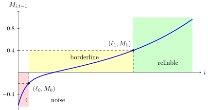
The margins of the objects of the training sample, ordered in ascending order (a schematic). The next base algorithm is trained only on the borderline objects, ; the noise () and reliable () objects do not enter its training sample.
How the subsample is formed is simplest to show in a picture. We take the margins of the objects and order them in ascending order. On the right is a region that does not interest us: on all these objects the composition is already good, and even if the next base algorithm errs there, the margin will not sag to zero; all will be well. On the left is a region that does not interest us either: these are noise objects, on which one should not even try to make a good positive margin. Everything is bad on them, and it will stay bad, it will not get better, so we simply get rid of these objects. And it turns out that by the margin criterion the middle region remains, the borderline objects; these are precisely the objects on which the next base algorithm should be trained. One could also build randomisation, the idea of bagging, into this, but we did not do that.
Definition (The principle of evening out the distribution of margins). Let us order the objects in ascending order of the margins . Two cases where should not be trained on the object :
- , : the object is noise;
- , : the object is reliable.
This is the pseudocode we got; we called this method ComBoost, committee boosting. What else is done here: when we train the next base algorithm, let us vary the size of the training sample. After all, we do not know exactly where on this distribution the noise objects ended and where the boundary between the borderline and the reliable ones runs; perhaps more of the reliable ones should be taken in. Let us make a whole series of training samples, build several base algorithms on them and choose the best of them as the next base algorithm of the composition.
Definition (The ComBoost algorithm (Committee Boosting)). Input: samples , ; parameters , , , , .
Output: .
- ; margins , ;
- for all , while improves substantially:
- order the sample in ascending order of the margins ;
- for all with step :
- ;
- , incremental training;
- choose the best by the criterion ;
- update the margins: , .
A. A. Matsenov. Committee boosting: minimising the number of base algorithms with simple voting // MMPR-13, 2007 (in Russian).
That is the whole idea. It turned out to be enough to minimise the number of base algorithms and to use fairly strong methods, such as SVM, as the base ones. On several problems from the UCI repository it was shown that substantially fewer base algorithms are really needed: sometimes one can manage with literally a few of them. This is a rather old work of ours, done by my graduate student A. A. Matsenov.
Example (The results of an experiment on 4 problems from the UCI repository). The percentage of errors on validation, over 50 random "training : validation" splits ; in brackets, the number of base algorithms .
| ionosphere | pima | bupa | votes | |
|---|---|---|---|---|
| SVM | 12.9 | 24.2 | 42.0 | 4.6 |
| ComBoost₀[SVM] | 12.6 (4) | 23.1 (2) | 34.2 (5) | 4.0 (2) |
| ComBoost[SVM] | 12.3 (5) | 22.5 (2) | 30.9 (5) | 3.8 (3) |
| AdaBoost[SVM] | 15.0 (65) | 22.7 (18) | 30.6 (15) | 4.0 (8) |
| Parzen | 6.3 | 25.1 | 41.6 | 6.9 |
| ComBoost₀[Parzen] | 6.1 | 25.0 | 38.1 | 6.8 |
| ComBoost[Parzen] | 5.8 | 24.7 | 30.6 | 6.2 |
| AdaBoost[Parzen] | 6.0 | 24.8 | 30.5 | 6.5 |
ComBoost₀ is without choosing the length of the subsample in the loop ; Parzen is the Parzen window method with the window width chosen by leave-one-out.
The result: ComBoost is able to build short ensembles of strong and stable base algorithms.
Conclusions
- Ensembles allow solving complex problems that individual base algorithms solve poorly.
- Usually an ensemble is built by a wrapper (envelope) algorithm: the base algorithms are trained by ready-made methods.
- Base algorithms: a quality/diversity trade-off.
- The two main heuristics of boosting (and not only of AdaBoost):
- train the base algorithms one at a time;
- use a smooth replacement of the threshold loss function.
- An important discovery of the mid-90s: the generalisation ability of boosting does not deteriorate with the growth of the complexity .
- A practical comparison of boosting and bagging:
- boosting is better for classes with boundaries of complex shape;
- bagging is better for short training samples;
- bagging is easier to parallelise.
No comments yet
Be the first to share your thoughts.