August 30, 2026 · Lecture · LibreTimes
Machine Learning 1. Lecture 15. A Short Review of the Semester
Contents
- What this lecture is about
- Types of optimisation problems in machine learning
- Empirical risk minimisation
- Underfitting, overfitting and regularisation
- Supervised learning
- Unsupervised learning
- Constructing models: six scientific schools
- The main scientific schools
- Symbolism
- Evolutionism
- Analogism
- Bayesianism
- Connectionism
- Compositionism
- The practice of machine learning
- CRISP-DM: a standard for the data analysis process
- Preprocessing and vectorising data
- Postprocessing and quality evaluation
- The bottom line
What this lecture is about
The closing review gathers the semester's material into three pictures. The first is the optimisation picture: almost any machine learning problem is posed as empirical risk minimisation with regularisation, and problems differ in their loss functions and models. The second is historical and methodological: the models of machine learning grew out of several scientific schools, each with its own heuristic about how data are arranged. The third is practical: what the process of data analysis looks like from understanding the problem to deployment, and what in it gets automated.
Types of optimisation problems in machine learning
Empirical risk minimisation
Definition (The general formulation of most machine learning problems). Given: , the object space; , the training sample, the precedents; , , a parametric model, the hypothesis.
Find: , the parameter vector of the model .
The criterion of empirical risk minimisation (ERM):
where is the loss function, the larger the worse the model's answer on the object ; is the regulariser, requirements on the model that do not come from the precedents; is the regularisation coefficient that balances the criteria.
This is the "DNA" of a problem — given, find, criterion — with which the solution of any problem begins. The loss function expresses what is known from the precedents; the regulariser, requirements on the model that do not follow from the precedents: smoothness, sparsity, small weights.
Definition (The gradient method of empirical risk minimisation). Gradient descent (GD):
where is the gradient vector and is the gradient step, also called the learning rate:
Stochastic gradient (Stochastic Gradient, SGD):
In the stochastic gradient each step takes one random object (or a small batch of objects) instead of the whole sample. A step becomes times cheaper, and its direction coincides with the gradient only on average; on large samples this pays off. This method is the main training tool, from linear models to deep neural networks.
Underfitting, overfitting and regularisation
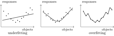
Underfitting (too simple a model), the right complexity, and overfitting (the model passes through every point but describes the dependency poorly).
Remark (The fundamental problems: underfitting and overfitting).
- Underfitting: there is plenty of data, too few parameters, the model is simple and inflexible.
- Overfitting: there are many parameters, too little data, the model is complex and excessively flexible.
As the complexity of a model grows, the error on the training sample falls monotonically, while the error on new data first falls and then grows. Between underfitting and overfitting lies a model of the right complexity; finding it, limiting complexity, and training complex models so that they do not overfit is a theme running through the whole course.
Definition (Multicollinearity and overfitting in linear models). Multicollinearity is a linear dependence between features:
- a linear regression or classification model ;
- multicollinearity: ;
- the solution is not unique: .
Multicollinearity leads to overfitting:
- instability: weights that are too large and of different signs;
- the weight cannot be interpreted as the importance of the feature ;
- overfitting: .
How to reduce overfitting:
- regularisation (weight decay);
- feature selection: , ;
- feature transformation: , .
If the features are linearly dependent, any multiple of the vector can be added to the weight vector without changing the model's answers on the training objects. The solution is no longer unique, and a numerical method can drift into a region of huge weights of different signs that cancel each other on the training sample but not on new data. The three remedies correspond to three lectures of the course: regularisation, feature selection, feature transformation (principal component analysis).
Definition (A penalty on model complexity reduces overfitting). A regulariser is an additive term to the main criterion, where is the regularisation coefficient, a control parameter:
regularisation of linear models :
- (Ridge, SVM) stabilises under multicollinearity;
- (LASSO) and lead to the selection of informative features.
Probabilistic regularisation (Maximum a Posteriori Probability):
Definition (Non-smooth regularisers for feature selection and grouping). The general form of the regularisers ( is the selectivity parameter):
Regularisers with feature selection and grouping effects:
- LASSO (): ;
- Elastic Net: ;
- Support Feature Machine (SFM):
- Relevance Feature Machine (RFM): .
Non-smoothness at zero is what gives feature selection: with a regulariser that has a kink at zero, the minimum of the criterion is often attained exactly at , and the corresponding feature drops out of the model. Elastic Net and SFM combine the kink at zero with quadratic growth away from zero, which makes it possible to select whole groups of correlated features rather than one random member of each.
Supervised learning
Definition (Training a regression model). Given: a training sample with responses .
Find: the parameter vector of a regression model .
Criterion: minimum empirical risk
with a unimodal loss function of the residual .
Unimodal loss functions for regression (slide): quadratic and robust; absolute, quantile and SVM.
The quadratic loss corresponds to the least squares method and Gaussian noise; the absolute loss to the least absolute deviations method and the median; the quantile loss to quantile regression; the SVM loss does not penalise small residuals; robust functions limit the influence of large residuals, that is, of outliers.
Definition (Training a binary classifier). Given: a training sample , .
Find: the vector of a classification model .
Criterion: minimum approximated empirical risk
with a decreasing loss function of the margin .
Decreasing loss functions for classification (slide): sigmoid, logistic, SVM hinge; exponential, quadratic, robust. In grey, the threshold function .
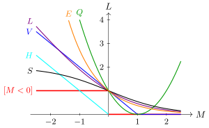
The threshold loss (red) and its continuous approximations: (SVM), , (logistic), , (sigmoid), (exponential).
The threshold loss — the number of errors — is piecewise constant and cannot be minimised by gradient methods. It is replaced by a continuous upper bound as a function of the margin; the choice of that bound is what produces the different methods: logistic regression, SVM, boosting (the exponential function) and others.
Definition (Training a multiclass classifier). Given: a training sample , , .
Find: the vector of a classification model .
The "one against one" criterion:
The "one against all" criterion:
where is the margin of the object with respect to the class .
Definition (Learning to rank, maximising AUC-ROC). Given: a training sample ; , the relation " is better than " between objects of .
Find: the parameters of a ranking model that recovers the correct order relation: .
Criterion: the number of wrongly ranked pairs of objects
where is a decreasing function of the pairwise margin .
Multiclass classification and ranking follow the same pattern: instead of the margin of an object there is the margin with respect to each other class, or the margin of a pair of objects, and the same decreasing loss function bounds the number of errors from above. The share of correctly ordered "positive–negative" pairs is AUC-ROC, so minimising such a criterion is a gradient method for maximising AUC.
Unsupervised learning
Definition (The density estimation problem). Given: , the training sample.
Find: the parameter vector of a generative model .
Criterion: maximum likelihood (MLE)
or maximum a posteriori probability — the joint likelihood of the data and the model with a prior density (MAP):
where is the vector of hyperparameters of the prior distribution.
Definition (The problem of estimating a mixture of densities). Given: , the training sample.
Find: the parameters , of a mixture model of probability distributions
Criterion: maximum likelihood or maximum a posteriori probability (MAP):
Minus the log-likelihood of an object is the same loss function, and the log of the prior distribution is the same regulariser: probabilistic formulations fit into the general scheme of empirical risk minimisation. Mixtures of distributions are solved by the EM algorithm.
Definition (The clustering problem). Given: , the training sample, .
Find: the cluster centres — parameters , — and a cluster for each object .
Criterion: minimum sum of within-cluster distances
the metric is usually Euclidean (but may be another): .
Definition (One-class SVM (OSVM)). Given: a training sample .
Find: the centre and the radius of a ball enclosing the whole sample except the anomalous outlier objects.
Criterion: minimise the radius of the ball and the sum of penalties for leaving the ball:
With the properties of the solution are similar to SVM: a convex quadratic programming problem; the solution is sparse and depends only on the support objects; generalisation to nonlinear models: .
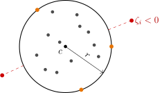
One-class SVM (schematic): a ball with centre and radius ; the orange objects on the boundary are the support objects, the red ones outside the ball are outliers.
Definition (The semi-supervised learning problem (SSL)). Given: , the labeled objects (labeled data) with labels , ; , the unlabeled objects (unlabeled data).
Find: a classification model .
The criterion of simultaneous classification and clustering:
where is the classification loss function and is the loss function for unlabeled data. The essence of SSL is the common parametrisation in the two criteria.
Definition (A special case of SSL: PU-learning (Positive and Unlabeled)). Examples of problems where objects of only one class are known: detecting fraudulent transactions; recommender systems, ad personalisation; automatically extending a knowledge base with facts.
A two-class classification model . Unlabeled objects are treated as negative with weight :
One can take only part of the unlabeled objects (negative sampling). One of the successful methods is Biased SVM.
Gang Li. A Survey on Positive and Unlabelled Learning. 2013. J. Bekker, J. Davis. Learning From Positive and Unlabeled Data: A Survey. 2020.
Definition (Principal Component Analysis (PCA)). Given: a sample of objects ; , numerical features of the objects.
Find a feature transformation: , new numerical features, , and a linear reconstruction of the old features from the new ones:
Criterion: the accuracy of reconstructing on the training sample:
where , .
Definition (The autoencoder: learned vectorisation). Given: , the training sample.
Find a vectorisation model that preserves information: , the encoder, with code vector ; , the decoder, with reconstruction .
The criterion of the quality of reconstructing the objects, :
The loss function may be quadratic: .
Example. PCA is a linear autoencoder: , , , . With the data about the objects are compressed.
Principal component analysis is a special, linear case of the autoencoder. If the encoder and the decoder are neural networks, the result is a nonlinear learned vectorisation, one of the central mechanisms of deep learning, to which the second half of the course is devoted.
Definition (The autoencoder: learned vectorisation for SSL). Data: labeled , unlabeled .
Find: , the encoder; , the decoder; , the predictor.
Loss functions are given: for reconstruction; for prediction.
Criterion: joint training of the autoencoder and the predictive model (classification, regression or other):
Dor Bank, Noam Koenigstein, Raja Giryes. Autoencoders. 2020.
Here again the principle of semi-supervised learning is at work: two criteria, on all the data and on the labeled data, with a common part of the parameters, the encoder . The unlabeled data train the vectorisation; the labeled data train prediction from the vector representations.
Constructing models: six scientific schools
The main scientific schools
Definition (The main scientific schools of machine learning).
- Symbolism: searching for logical regularities: Decision Tree, Rule Induction.
- Evolutionism: self-development of complex models: Genetic Algorithms, Genetic Programming, Symbolic Regression.
- Analogism: "close objects have close answers": kNN, RBF, SVM, Kernel Smoothing.
- Bayesianism: estimating the distributions of parameters: Naive Bayes, Bayesian Networks, Graphical Models.
- Connectionism: training neural networks: BackPropagation, Deep Belief Nets, Deep Learning.
- Compositionism: cooperation of models: Weighted Voting, Boosting, Bagging, Stacking, Random Forest, CatBoost.
Pedro Domingos. The Master Algorithm. 2015.
Pedro Domingos identified five schools in his book "The Master Algorithm"; the sixth, compositionism, is added to them because ensembles of models form an independent direction. Each school rests on its own heuristic about how data are arranged, and many of the schools have strong Soviet roots.
Symbolism
Definition (Symbolism. The scientific school of M. M. Bongard).
- 1958: the program "Discover the Law" recovered a dependency by exhaustive combinatorial search over formulas.
- 1959: the program "Arithmetic" used informativeness estimates to cut the search.
- 1961: the program "KoRa" searched over informative triples of features.
"KoRa-3" was the first application of the recognition of non-visual patterns: recognising the oil–water boundary in a well. It introduced the principles of voting and cross-validation, and the notions of informativeness and of prejudice (overfitting).
M. M. Bongard, M. N. Vaintsvaig, Sh. A. Guberman, M. L. Izvekova, M. S. Smirnov. The use of a learning program for detecting oil-bearing strata. 1966 (in Russian).
Definition (The notion of an informative logical regularity). The classification model is a weighted vote of rules:
A rule is a conjunction of elementary threshold conditions:
A syndrome: at least conditions of the set hold:
A rule is a regularity of the class if
Symbolism means the logical methods of classification: decision trees, decision lists and rule sets. A regularity must pick out many objects of its own class and few of the others; the two-criterion nature of this requirement produces the various informativeness criteria.
Evolutionism
Definition (Evolutionism. Algorithms that search over model structures). Discrete optimisation based on Darwinian evolution:
- an individual is a structural formula of a model;
- a population is a set of different formulas;
- fitness is an external criterion, an evaluation of the model;
- natural selection of the best models in the population;
- crossover and mutation are the operations that produce offspring.
Particular machine learning problems solved by evolutionary algorithms:
- feature selection;
- searching for informative logical regularities;
- searching for the architecture of a deep neural network;
- symbolic regression: a search over structural formulas, genetic programming.
Definition (Evolutionism. The scientific school of A. G. Ivakhnenko). The group method of data handling (GMDH) is based on the self-organisation of models, a search-based optimisation of the model structure:
- selection of features or of the model structure;
- during the search the quality of the models is assessed by many external criteria: cross-validation, noise immunity of the modelling, balance (consistency) of forecasts, and others;
- the first 8-layer deep neural network (1965);
- hundreds of applications, about 300 dissertations.
A. G. Ivakhnenko, V. G. Lapa. Cybernetic Predicting Devices. 1965. A. G. Ivakhnenko, Yu. P. Zaichenko, V. D. Dimitrov. Decision Making Based on Self-Organisation. 1976. A. G. Ivakhnenko. An Inductive Method of Self-Organisation of Models of Complex Systems. 1982 (all in Russian).
The key idea of GMDH is external criteria: a model is evaluated not on the sample it was trained on but on a control one, and this makes it possible to search over model structures without overfitting at the selection stage. The same idea underlies cross-validation and the model selection methods of the lecture on quality.
Analogism
Definition (Analogism. The scientific school of M. A. Aizerman).
- The compactness hypothesis: similar objects as a rule lie in the same class.
- The method of potential functions: the idea is borrowed from physics.
- A linear classification model: a weighted vote of the similarity functions between and :
M. A. Aizerman, E. M. Braverman, L. I. Rozonoer. Theoretical foundations of the potential function method in the problem of teaching automata to classify input situations. 1964. M. A. Aizerman, E. M. Braverman, L. I. Rozonoer. The Method of Potential Functions in the Theory of Machine Learning. 1970. A. G. Arkadiev, E. M. Braverman. Teaching Machines to Recognise Patterns. 1964 (all in Russian).
The method of potential functions is already a linear classifier in the space of similarity functions to the objects of the sample, that is, in essence, a kernel method: thirty years later the same construction appeared in SVM with kernels.
Definition (Analogism. Metric (nonparametric) methods). Density estimation. The Parzen–Rosenblatt method:
Classification. Potential functions, the Parzen window:
Regression. Nadaraya–Watson kernel smoothing:
One and the same construction — a kernel of the distance divided by the window width — gives a method for three different problems: density estimation, classification and regression.
Definition (The principles of learnability, complexity limitation, separability). A family of classifiers is learnable if
where is the error probability of the classifier and is the empirical risk, the error rate of the classifier on the sample.
The main results of VC theory:
- a justification for limiting the complexity of ;
- the notion of the capacity of a family, VCdim;
- the method of structural risk minimisation;
- the support vector machine, SVM.
V. N. Vapnik, A. Ya. Chervonenkis. Theory of Pattern Recognition. Moscow: Nauka, 1974 (in Russian).
The Vapnik–Chervonenkis theory gave a mathematical justification for the principle of limiting model complexity: if the capacity of the family is small compared with the sample length, the error rate in training is uniformly close to the error probability. Structural risk minimisation and the support vector machine grew out of it.
Bayesianism
Definition (Discriminative and generative classification models). Given: a simple sample .
The discriminative approach: find a model (examples: LR, GLM, SVM, RBF). The maximum likelihood criterion:
The generative approach: find a model (examples: NB, PW, FLD, RBF). The maximum likelihood criterion:
The discriminative approach models only what classification needs, the conditional probability of the class. The generative one recovers the distribution of objects within each class and obtains a classifier through Bayes' formula; it needs more assumptions, but it makes it possible, for example, to generate objects and to detect atypical ones. The RBF network appears in both lists: it can be trained both as an SVM with a radial kernel and by the EM algorithm as a mixture of Gaussians.
Definition (Bayesian learning, MAP and regularisation). Bayesian inference of the posterior distribution and a point estimate:
Maximising the posterior probability (MAP) gives a point estimate of directly, without inferring the Posterior:
Regularisation, not necessarily probabilistic:
Three levels of rigour: full Bayesian inference of the posterior distribution, a point estimate of its maximum, and regularisation, which may have no probabilistic interpretation at all. A Gaussian prior gives the regulariser, a Laplace prior the one.
Connectionism
Definition (Connectionism. The linear model of a neuron (1943)).
where are the features of the object ; are the feature weights; is the activation threshold; is the activation function.
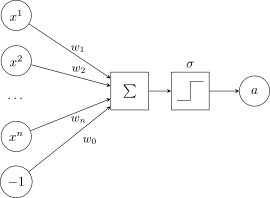
The McCulloch–Pitts neuron: the feature values enter with weights , the threshold as the weight of a constant input ; the sum passes through the activation function .
The neuron model of Warren McCulloch and Walter Pitts (1943) is a linear classifier with an activation function. Multilayer networks are built from such neurons.
Remark (Rosenblatt's perceptron (1957) and milestones in the development of neural networks).
- F. Rosenblatt's perceptron (1957): a two-layer network trained by error correction; Mark-1, the first neurocomputer (1960), for recognising digits and shapes. F. Rosenblatt. Principles of Neurodynamics: Perceptrons and the Theory of Brain Mechanisms. 1962.
- M. Minsky, S. Papert. Perceptrons. 1969.
- A. G. Ivakhnenko, V. G. Lapa. Cybernetic Predicting Devices. 1965 (in Russian).
- A. I. Galushkin. Synthesis of Multilayer Pattern Recognition Systems. 1974 (in Russian).
- Rumelhart D. et al. Learning internal representations by error propagation. 1986.
- Krizhevsky A. et al. ImageNet classification with deep convolutional neural networks. 2012.
- Vaswani A. et al. Attention is all you need. 2017.
The history of neural networks knows periods of rapid development and "winters" (AI winters). The book by Minsky and Papert showed the limitations of the single-layer perceptron and cooled interest in neural networks for years; multilayer networks and the backpropagation method (in the Soviet literature, A. I. Galushkin, 1974; widely known from the work of Rumelhart and co-authors, 1986) brought it back; the deep convolutional networks of 2012 and the transformer architecture of 2017 opened the present stage.
Remark (Deep convolutional networks for image classification). The ImageNet competition started in 2009; the human error level of 5% was passed in 2015. Convolutional neural networks: AlexNet (2012), ResNet (2015).
Li Fei-Fei et al. ImageNet: A large-scale hierarchical image database. 2009. Krizhevsky A. et al. ImageNet classification with deep convolutional neural networks. 2012. Kaiming He et al. Deep residual learning for image recognition. 2015.
The development of machine and deep learning is conveniently described in three stages, by the type of a model's input and output.
Stage 1: vector → scalar (slide). Predictive modelling of vector data.
Definition (Stage 1: vector → scalar). Predictive modelling of vector data. Input: vector feature descriptions of objects. Output: scalar answers (predictions, forecasts).
Applications: medical diagnosis, geological forecasting, credit scoring…
Models: SVM, LR, MVR, RBF, MLP, ID3, CART, RF, GBM…
Stage 2: structure → vector → scalar (slide). Learned vectorisation of complexly structured data.
Definition (Stage 2: structure → vector → scalar). Learned vectorisation of complexly structured data. Input: the complexly structured "raw" data of objects. Output: vector representations of objects, then answers.
Applications: classification of images, texts, signals, voice commands, biometric identification of persons…
Models: CNN, AlexNet, ResNet, word2vec, FastText, BERT…
Stage 3: structure → vector → structure (slide). Learned generation of complexly structured data.
Definition (Stage 3: structure → vector → structure). Learned generation of complexly structured data. Input: complexly structured objects. Output: complexly structured answers.
Applications: image captioning and synthesis, style transfer, speech recognition, machine translation, text summarisation, chatbots with emergent abilities…
Models: seq2seq, RNN, LSTM, GAN, VAE, GPT…
At the first stage a person built the features, and the model mapped the feature vector to an answer. At the second, the vectorisation of complex objects — images, texts, signals — became a learned part of the model. At the third, the model also learned to generate complexly structured objects from their vector representations.
Compositionism
Definition (The problem of training an ensemble (composition) of models). Given: , the training sample; , "weak" trainable base models; , algorithmic operators with parameters ; , a decision rule of a simple form (without parameters); , a convenient space of estimates.
Find: an ensemble , where is a correcting function with parameters .
The criterion for training a "strong" algorithm as an ensemble of base algorithms that are "weak" taken separately:
Yu. I. Zhuravlev. On an algebraic approach to solving recognition or classification problems. Problemy Kibernetiki, 1978 (in Russian). M. Kearns, L. G. Valiant. Cryptographic limitations on learning Boolean formulae and finite automata. 1989.
Definition (Examples of correcting (aggregating) functions).
- Simple voting: .
- Weighted voting: , , .
- Feature-weighted linear stacking: , .
- A mixture of experts with competence functions (gating functions) : .
Definition (Training predictive models and their ensembles). is the loss function of the model given the answer .
Empirical risk minimisation for the base algorithms:
Empirical risk minimisation for adding a base algorithm to the ensemble, with the previous ones fixed:
Yu. I. Zhuravlev. Correct algebras over sets of incorrect (heuristic) algorithms (I, II, III). Kibernetika, Kiev, 1977–1978 (in Russian). Y. Freund, R. E. Schapire. A decision-theoretic generalization of on-line learning and an application to boosting. 1995. K. V. Rudakov, K. V. Vorontsov. On methods of optimisation and monotone correction in the algebraic approach to the recognition problem. Doklady RAN, 1999 (in Russian).
Adding base algorithms one at a time, with the previous ones fixed, is the scheme of boosting; in the simplest case each base algorithm is trained separately and then combined by voting, as in bagging and random forests. Yu. I. Zhuravlev's algebraic approach to building correct algorithms out of incorrect heuristic ones was more than a decade ahead of Kearns and Valiant's notion of weak learning and of Freund and Schapire's boosting.
Definition (Estimate-calculating algorithms, ECA (Yu. I. Zhuravlev)). A union of the main non-rigorous (heuristic) principles of the time:
- symbolism (deriving rules from data);
- evolutionism (selecting the best rules);
- analogism (estimates of the similarity of objects);
- Bayesianism (classes are mixtures of densities);
- connectionism (weighted voting).
where are binary similarity functions over feature subsets :
Yu. I. Zhuravlev, V. V. Nikiforov. Recognition algorithms based on the calculation of estimates. 1971 (in Russian).
ECA as a three-layer RBF network (slide): .
Remark (ECA unites many heuristic principles).
- a three-layer RBF (radial basis function) neural network;
- the method of potential functions: ;
- a linear SVM classifier with a radial kernel;
- a Bayesian classifier with mixture densities ;
- prototype selection: for non-prototypes ;
- feature selection in spherical logical regularities.
Estimate-calculating algorithms are an example of a model that as early as 1971 united the approaches of almost all the schools: estimates of similarity to prototypes over subsets of features, their voting, selection of prototypes and of features.
Definition (The principles of informativeness, consistency, irreducibility).
- The informativeness of a predicate for a class :
- The informativeness of a similarity function :
- Consistency: , :
- a test : for all such that ;
- a representative set : for all such that .
- Irreducibility: no subset of features is a test (or a representative set).
A. N. Dmitriev, Yu. I. Zhuravlev, F. P. Krendelev. On a principle of classification and forecasting of geological objects and phenomena. 1968. Yu. I. Zhuravlev, V. V. Nikiforov. Recognition algorithms based on the calculation of estimates. 1971 (both in Russian).
Example (Problems on small data). Features of geological data in the search for deposits of a rare type (gold, uranium, diamonds, etc.):
- few objects (), many features (more than a hundred);
- there is no reliable geophysical model;
- the data have gaps, unmeasured values.
F. P. Krendelev, A. N. Dmitriev, Yu. I. Zhuravlev. A comparison of the geological structure of foreign deposits of Precambrian conglomerates by means of discrete mathematics. Doklady AN SSSR. 1967. A. N. Dmitriev, Yu. I. Zhuravlev, F. P. Krendelev. On a principle of classification and forecasting of geological objects and phenomena. 1968 (both in Russian).
Tests and irreducible representative sets were born of such problems: with eighteen objects and a hundred features, statistical methods are powerless, and classification has to be built on combinatorial principles, by searching for minimal consistent feature sets that distinguish objects of different classes.
The practice of machine learning
CRISP-DM: a standard for the data analysis process
Definition (A cross-industry standard for data mining). CRISP-DM (CRoss Industry Standard Process for Data Mining, 1999). Initiating companies: SPSS, Teradata, Daimler AG, NCR Corp., OHRA.
Steps of the process:
- business understanding;
- data understanding;
- data preprocessing and feature engineering;
- model development and parameter tuning;
- quality evaluation;
- deployment.
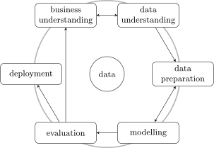
The CRISP-DM cycle (schematic): six steps around the data; business understanding and data understanding, data preparation and modelling refine each other, and evaluation can send the process back to business understanding.
Definition (The evolution of AI as the automation of CRISP-DM steps).
- Expert Systems: rigid rule-based models.
- Machine Learning: parametric models trained on data.
- Deep Learning: models with learned vectorisation of the data.
- AutoML: automatic selection of models and of their structure.
- Lifelong Learning: seamless integration into the business process.
Each stage in the development of artificial intelligence automates the next step of the process: machine learning replaced the manual construction of rules by experts with modelling from data; deep learning joined feature preparation to modelling; AutoML automates model selection and evaluation; lifelong learning builds all of this into deployment.
Preprocessing and vectorising data
Definition (Features of the data and of the formulations of applied problems). Data can be:
- heterogeneous (features measured on different scales);
- incomplete (not everything was measured, there are gaps);
- inaccurate (measured with errors);
- contradictory (identical objects, different answers);
- excessive (very large, does not fit in memory);
- insufficient (fewer objects than features);
- complexly structured (no feature descriptions).
Risks associated with the problem formulation:
- "dirty" data (the customer does not ensure data quality);
- unclear criteria of model quality (the customer has not settled on goals or criteria).
Definition (Data preprocessing methods).
- Feature transformation: strengthening or weakening the measurement scale of a feature; normalisation, standardisation; transforming the distribution function of a feature.
- Feature extraction from raw data, feature engineering.
- Representation learning, learned vectorisation of data.
- Missing values imputation.
- Outlier / anomaly detection.
- Dimensionality reduction.
- Feature selection, choosing the informative features.
Postprocessing and quality evaluation
Definition (Model evaluation and selection problems). Given: , the training sample; , parametric models, ; , the parameter space of the model ; , learning methods, .
Find: the method with the best generalisation ability.
Special cases:
- choosing the best model (model selection);
- choosing the learning method for a given model (in particular, hyperparameter optimisation);
- feature selection: is the set of features; the learning method uses only the features .
Definition (The methodology of error (or loss) analysis). is the loss function (the smaller the better). The mean loss on a sample and its empirical distribution:
Analysing losses on the training sample:
- rank the objects by decreasing loss ;
- are the objects with extremely large losses outliers?
- if not, how can the model be improved on these objects?
Comparing losses in training and on test:
- do the loss distributions differ much?
- if they do, how can overfitting be eliminated?
One number, the average quality, is not enough. The distribution of losses over objects shows where the model errs: on a few outliers, or systematically on a whole group of objects; and comparing the distributions in training and on test shows whether there is overfitting and on which objects it shows up.
Definition (A/B testing (split testing)). Two models, "baseline A" and "improved B", built from historical data , are tested by a quality metric on new data .
How does A/B testing differ from an ordinary hold-out?
- is genuinely future data (out-of-time), not part of the past data excluded from training (out-of-sample);
- more realism: the properties of the data stream may change over this time, real data need not be i.i.d.;
- a one-off choice of model hardly overfits;
- accumulating the data may take a long time;
- the model's operation may affect how the data stream is formed (in recommender systems, for example).
Definition (Meta-learning (learning to learn)). The problem: too many methods, too long to run.
Given: a sample of "problem, method" → quality criteria.
Find: a multiclass classification model that predicts which method to solve a problem with.
Criterion: the accuracy of predicting the optimal method.
Features: the size characteristics of the problem; characteristics of the feature space — types, outliers, gaps, correlations; the results of fast low-dimensional methods.
Joaquin Vanschoren. Meta-learning Architectures: Collecting, Organizing and Exploiting Meta-knowledge. 2009. Joaquin Vanschoren. Meta-Learning: A Survey. 2018.
Definition (Automatic selection of models and hyperparameters (AutoML)). The problem: choosing the model structure (the architecture of a neural network) and the hyperparameters takes too many resources.
Given: a sample of "problem, structure" → quality criteria.
Find: which experiment to run next with the model.
Criterion: minimise the resources spent on an automatic search for an optimal model comparable in quality to models built by professional researchers.
A close classical problem is experiment design.
Xin He et al. AutoML: A Survey of the State-of-the-Art. 2019.
Meta-learning and AutoML are machine learning applied to the process of machine learning itself: the objects become problems and experiments, and the answers the quality of the methods on them.
The bottom line
Remark (The bottom line).
- We start with the problem formulation: the DNA (given, find, criterion).
- P. Domingos (2015) was wrong that the "master algorithm" (AGI) would appear as a union of the approaches of the main scientific schools.
- Yu. I. Zhuravlev had already done that in the estimate-calculating algorithms (1971), but it did not lead to AGI.
- It is now clear that the ingredients of success are quite different:
- learned vectorisation of data → deep learning;
- big data + big models + neural processors;
- high dimensions + optimisation without overfitting;
- large language models → emergence.
Literature
- K. V. Vorontsov. Lectures on Machine Learning (in Russian).
- S. Nikolenko. Machine Learning: Foundations. 2025 (in Russian).
- K. P. Murphy. Probabilistic Machine Learning: An Introduction. 2022; Probabilistic Machine Learning: Advanced Topics. 2023.
- M. P. Deisenroth, A. A. Faisal, C. S. Ong. Mathematics for Machine Learning. 2020.
- Christopher Bishop, Hugh Bishop. Deep Learning: Foundations and Concepts. 2024.
- S. Markov. Hunting Electric Sheep: The Big Book of Artificial Intelligence. 2024 (in Russian).
- P. Domingos. The Master Algorithm: How the Quest for the Ultimate Learning Machine Will Remake Our World. 2015.
No comments yet
Be the first to share your thoughts.