August 30, 2026 · Lecture · LibreTimes
Machine Learning 1. Lecture 12. Density Estimation and Bayesian Classification
Contents
- What this lecture is about
- Parametric density estimation
- The maximum likelihood principle
- The multivariate Gaussian density
- The geometric meaning
- The multicollinearity problem
- Separating a mixture of distributions
- A mixture of distributions
- The EM algorithm
- A mixture of Gaussians (GMM)
- Nonparametric density estimation
- The one-dimensional case
- The Parzen–Rosenblatt estimate
- The multivariate case
- The choice of kernel
- The choice of window width
- A retrospective: three problems with one construction
- Three approaches to density estimation
- Bayesian classification theory
- Generative models of classification
- The discriminative and generative approaches
- The optimal Bayes classifier
- A survey of Bayesian classifiers
- The Parzen window method
- The quadratic discriminant
- Fisher's linear discriminant
- Gaussian mixtures and the radial basis function network
- Where this is applied
- Conclusions
- Seminar
What this lecture is about
The course programme actually has two lectures here: one on density estimation on its own, the other on Bayesian classification theory on its own. They are closely related things, so this semester I merged them, but the merged lecture bears the traces of the merger: it has come out large, and some things I will tell in less detail or leave out. That should not affect the general understanding.
Today it is the problem of estimating a probability density, and we will look at three main approaches: the classical parametric one, mixtures of distributions, and the nonparametric one. Then, on the basis of these approaches, we will see how classification algorithms are built.
Parametric density estimation
The maximum likelihood principle
Suppose we have a sample. This is unsupervised learning: there are objects, but there are no answers for them, only . It is assumed that these came from some density , and this density has to be recovered: we have to understand which density the observed objects of the sample came from.
Definition (The density estimation problem (unsupervised learning)). Given: a simple (i.i.d.) sample .
Find: a parametric model of the probability density
where is a vector of parameters and is a fixed function.
Criterion: the method of maximum likelihood of the sample (Maximum Likelihood Estimate, MLE, maximum log-likelihood):
Analytical solution: the necessary condition for an extremum
provided the function is sufficiently smooth in .
The first thing that comes to mind: let us describe the density by a parametric family of functions. Say we know the form of the dependence, but the parameters are unknown. This is very much like the way we solve classification and regression problems: we fix a dependence with parameters and train the parameters. But we have to understand by what criterion to train, and here mathematical statistics comes to our aid, telling us that such a problem should be solved by the maximum likelihood principle. We write out the probability density of the whole sample: it is the product of the one-object densities. We are entitled to write a product because there is the i.i.d. assumption, independent identically distributed, a simple sample: the observations appear independently of one another from one and the same density. The logarithm is a monotone function, so we may maximise the logarithm. And if we are used to minimising a loss function, then our loss function is minus the logarithm of the density model. The problem has again been reduced to optimisation, and numerical methods can be used. But let me tell you about the classical situation where this problem can be solved analytically.
The multivariate Gaussian density
Example (The multivariate Gaussian density). Given: a sample generated by a Gaussian density:
Find the parameters of the distribution:
- , the expectation vector, ;
- , the covariance matrix, , symmetric, non-singular, positive definite.
Criterion: the maximum of the (log-)likelihood of the sample.
Sample maximum likelihood estimates:
This is the multivariate Gaussian distribution. Why the density formula is like this is material for another course, mathematical statistics; for us it is a working tool. The function is given up to its parameters: is the expectation vector, the covariance matrix. We have to learn to estimate them from the sample, of course by the maximum likelihood principle. For that the function has to be carefully differentiated with respect to the parameters, and . is a vector, and we know how to differentiate with respect to a vector, but is a covariance matrix, a symmetric one at that, so differentiating with respect to it is not a very simple undertaking. There is an inverse matrix in there, and the determinant of in the denominator, and one has to learn to differentiate a scalar function, the density, with respect to such expressions. We will skip these technical details now; the proofs are textbook ones and are given in many places. The main thing is that the result is very clear and predictable.
The sample estimate of the expectation vector is, of course, the mean over all the objects of the sample: the centre of the sample is easy to compute, we just average all the vectors . And the sample estimate of the covariance matrix is, as one would expect, this matrix: are the centred object vectors, and from each of them we made a matrix by multiplying a column by a row, the vector by itself. The sum of such matrices is the sample estimate of the covariance matrix.
The geometric meaning
The scatter ellipsoid of a multivariate normal density (slide). Left: , the axes of the ellipse are parallel to the unit vectors. Right: the general case; the axes of the ellipse are the eigenvectors of the matrix .
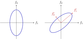
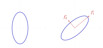
The scatter ellipsoid of a multivariate normal density. Left: , the axes of the ellipse are parallel to the unit vectors. Right: the general case; the axes of the ellipse are the eigenvectors of the matrix , and in the rotated coordinates the covariance matrix is diagonal.
Remark (The geometric meaning of the multivariate normal density). The scatter ellipsoid is a cloud of points of elliptical shape. When the axes of the ellipsoid are parallel to the unit vectors. In the general case is the spectral decomposition: are the orthogonal eigenvectors, ; are the eigenvalues of the matrix ;
where is an orthogonal transformation, a rotation or a reflection.
What a multivariate Gaussian density looks like you should also already understand from other courses; this is just a reminder. It is a swarm of points, an ellipse; it is called the scatter ellipsoid. One can show that the axes of this ellipse are connected with the orthogonal eigenvectors of the covariance matrix. We will not do that now; today's lecture does not use it specifically. But it is useful to illustrate the geometric meaning of the multivariate Gaussian, simply to picture it as a cloud of points of elliptical shape in the space , the space of object vectors.
The multicollinearity problem
Definition (The multicollinearity problem). The problem: when the matrix is singular, but even when it may turn out to be ill-conditioned.
Regularisation of the covariance matrix, , increases the eigenvalues by while keeping the eigenvectors (the parameter can be chosen by cross-validation).
Diagonalisation of the covariance matrix: the "naive" assumption that the features are independent leads to estimating one-dimensional densities of the features:
There is a little problem, of course: we are going to invert the covariance matrix, and it may turn out to be singular, and in some cases it will be singular with a guarantee. Let us look again at how the sample estimate of the covariance matrix is defined: it is the sum of matrices of rank one. Imagine the situation where the amount of data is less than the dimension of the vectors, that is, the number of features . You have added up matrices of rank one, and the rank of the resulting matrix cannot exceed ; it is of size , and there are not enough objects. Then the estimate of the covariance matrix is singular with a guarantee; it is a matrix of incomplete rank. And even if there are more objects than features, it may still turn out to be close to singular: there may be linear dependences among the features, multicollinearity. We have already discussed how to work with such things when we talked about regression. A slight modification of the covariance matrix is possible that at once makes it well-conditioned; one only has to choose the constant , the regularisation coefficient.
Let us look at the scatter ellipsoid again. Adding to the diagonal leads to every eigenvalue increasing by exactly , while the eigenvectors stay where they are: the scatter ellipsoid gets inflated a little, along every coordinate it grows by . What is multicollinearity in this geometric interpretation? It is an ellipse flattened along some coordinates right down to zero. And when you have inflated it by adding to each eigenvalue, the covariance matrix has ceased to be singular. That is the geometric meaning of regularisation: inflating the scatter ellipsoid.
Or one can do something quite radical and say: let the covariance matrix be diagonal altogether. On its diagonal are the variances of the features, and off the diagonal the covariances between features. If we assume that the features are independent, and for Gaussian distributions this is equivalent to their being uncorrelated, the problem becomes very much simpler: we no longer need to invert non-diagonal covariance matrices, and diagonal ones are easily inverted. Estimating an -dimensional density becomes a very simple problem: estimating one-dimensional densities. For each feature separately we compute the expectation and the variance: the ordinary familiar scalar estimates, the mean value of the feature over all objects and its variance. Of course, such an assumption rarely holds: in most problems one should hardly expect the features to be statistically independent. But the solution becomes much simpler: recovering one-dimensional densities is much easier than recovering one -dimensional density.
That is a short story about how density estimation problems are solved if we know the functional form of the density. Analytically the problem is solved neatly only for the normal density; for more complex forms of densities one has to use numerical optimisation.
Separating a mixture of distributions
Now let us consider another situation where there is a numerical method, but a specific one, very interesting and used in many places in machine learning. We will look at it now for separating a mixture of distributions. You have some data sample and do not believe that it is represented by a single scatter ellipsoid; you cannot describe it by one multivariate Gaussian density. But you suspect that there is a mixture of densities there: the complex shape of the sample is due to part of the data coming from one Gaussian density, part from another, part from a third. Though why Gaussian? Let us do it in general form.
A mixture of distributions
Definition (The problem of separating a mixture of distributions). Given: a sample generated i.i.d. from .
Find: a model of a probabilistic mixture of distributions
describing a two-level process that generates the data:
- , a discrete prior distribution;
- , the density of the -th component.
Criterion of maximum log-likelihood:
There are separate components , which are still probability densities, but there are several of them, and their probabilistic mixture with coefficients that are in essence a discrete probability distribution. The expression for a mixture of distributions describes a two-level generative model of the data. What does two-level mean? is generated in two steps. First, from the discrete distribution of the prior probabilities of the components, a kind of asymmetric coin or -sided die, you toss it and generate the number of a mixture component. Then you go to this component and generate itself from its distribution. Such two-stage schemes for generating objects are also called a generative story: a little tale of how the objects of the sample appear. They no longer come from one distribution but from a mixture of distributions.
A mixture of distributions is in fact also a parametric form of writing a distribution, only it has more parameters: now we have to estimate the parameters of each mixture component, and there are also the non-negative normalised prior probabilities of the components ; they have to be estimated too. If we write out the problem of maximising the log-likelihood, we get a very inconvenient functional, where there is a sum under the logarithm. Why was the problem solved analytically for the multivariate Gaussian distribution? Because it is exponential: the logarithm and the exponential immediately cancelled each other, and what was left was an expression that is easy to differentiate with respect to the model parameters, to get a system of equations and solve it. Here the sum under the logarithm at once cuts off every path to an analytical solution. Whichever way you turn it, a numerical method will have to be invented. One could, of course, solve this problem head-on with some stochastic gradient, but mankind has come up with a much more interesting way.
The EM algorithm
This way is called the EM algorithm, from the words expectation and maximization; that is what the two steps of this algorithm were called. It is an iterative process, and we will even prove a theorem now.
Theorem (Necessary conditions for an extremum). A point of a local extremum of satisfies a system of equations in the model parameters , and the auxiliary variables :
E-step:
M-step:
The EM algorithm is the method of simple iterations for solving this system.
The theorem gives necessary conditions for an extremum: the totality of all the parameters of the mixture at a point of local extremum of our functional, the log-likelihood, satisfies a system of equations in all the parameters. And the system of equations is written in such a fortunate way that it simply asks to be solved by the method of simple iteration: just compute the expressions on the left-hand side of the system by these formulas, variable by variable. We only have to explain what these auxiliary variables are. Looking at the formula, we see only that it is some function of the model parameters given by a not very complicated formula; it can be computed if and are known. That is, we have some initial approximation, from it we compute , and then, knowing , we can compute an approximation for and for . That is the whole method of solving this system of equations.
Remark (The probabilistic interpretation of the steps of the EM algorithm). The E-step is Bayes' formula:
the normalisation of the conditional probabilities: .
The M-step is the maximisation of the weighted log-likelihood with object weights for the -th mixture component:
the weight of a component is defined as the mean weight of its objects: .
Let us interpret this system, and then deal with the proof. It turns out that the E-step is simply Bayes' formula, and the have a very clear probabilistic interpretation: they are the posterior probabilities of the components for the objects of the training sample. The meaning is this: if we look at the -th object, with what probability could it have been generated by each, the -th, component? That is what we estimate, and those are our auxiliary variables. Why Bayes' formula? We simply write it out by the formula for conditional probability. Note that I denote probabilities by a capital and probability densities in the space by a small ; I always follow this mnemonic rule. The numerator turns out to be one term of our mixture of distributions and the denominator the mixture itself, and that is where the formula came from. So far this is only an interpretation; we will now prove this formula rigorously, and it will appear from the solution of the optimisation problem as if by itself.
And the M-step is the solution of a problem very similar to maximising the log-likelihood, written out separately for each component in terms of the hidden variables . These auxiliary variables show to what degree each object of the sample belongs to the -th component. Look: in the log-likelihood functional we took each -th object with a weight coefficient, the degree to which it belongs to the -th component. These weights are normalised over . If an object does not belong to the -th component at all, it will be removed from this sum, and in the sum we take only those objects that, as we estimated, were generated by the -th component. It turns out that the problem of estimating the parameters of a mixture of distributions has split into independent subproblems of estimating each component separately. The E-step estimated the degree to which an object belongs to each component, and then we know which objects each component consists of, and we estimate each component by maximum likelihood. That is, we have reduced the problem of estimating a mixture to a problem we can already solve after a fashion, and for Gaussian components can solve well.
Now the proof, literally in a couple of words, because we have no time today, and I want to tell you everything.
Proof. On there are equality and inequality constraints: is a discrete distribution, they are non-negative and sum to one. Because of these constraints we are forced to use the Karush–Kuhn–Tucker conditions and write out the necessary conditions for an optimum. We write out the Lagrangian of the optimisation problem : the main criterion and the dual variable for the equality constraint:
And where are the inequality constraints? A little trick: we can pretend they are not there, simply throw out , and later it will turn out that they are satisfied automatically, by themselves. This cannot always be done; here we were simply lucky; in this case it shortens the proof slightly.
We set the derivatives to zero. First with respect to :
A recognisable thing has formed here: that very auxiliary variable . Adding these equations over , we get ; we substitute it back and express . The probabilistic meaning is clear: we have averaged over all objects of the sample the degree to which the -th object belongs to the -th component, and this is an estimate of the prior probability of the component, its share in the whole sample. A perfectly reasonable interpretation.
Now let us differentiate with respect to . The trick: we divide and multiply by , and the derivative of divided by is the derivative of the logarithm:
We were lucky: exactly the same expression turned up here as in the first case. There are two main equations, for and for , and stood out as an auxiliary variable in both equations; we include it in the system and get what the theorem states.
The theorem does not in fact speak of an algorithm: it says that there is a system of equations, the necessary conditions for an extremum of the functional being optimised. It just happened to be written so, we were so lucky, that it can be solved by the method of simple iteration, and that method is what is called the EM algorithm. There are deeper proofs that this algorithm converges, unfortunately in a weak sense; there are no strong results about convergence for the EM algorithm, still less about global convergence. But the approach has proved very productive.
Definition (The EM algorithm for separating a mixture of distributions). Input: , .
Output: , the parameters of the mixture of distributions.
- initialise , ;
- repeat
- E-step (expectation): for all , : ;
- M-step (maximization): for all : ; ;
- until , and/or have converged.
Let us gather everything into one piece of pseudocode. There is some initialisation: we will probably initialise randomly, and for the prior probabilities of the components we take the uniform distribution. Then we repeat the E-step and the M-step until the parameters converge. At the E-step we estimate by Bayes' formula to what degree each -th object belongs to the -th component. The M-step is a decomposition: each component of the mixture is estimated separately.
A mixture of Gaussians (GMM)
Definition (Separating a mixture of Gaussians (Gaussian Mixture Model, GMM)). Input: , .
Output: , the parameters of the mixture of Gaussians.
- initialise , ;
- repeat
- E-step (expectation): for all , : ;
- M-step (maximization): for all :
- until and/or have converged.
If we substitute multivariate Gaussian distributions for , we get a very well-known variety of the EM algorithm: separating a mixture of Gaussians, the Gaussian Mixture Model, GMM. In general form is estimated as the solution of the problem of maximising the weighted log-likelihood, and it can be solved only when the concrete density is known. In the Gaussian case, fortunately, this problem is solved analytically: here are the analytical estimates for the expectation vector and for the covariance matrix. The summation here is over the whole sample, but with the weights : the -th mixture component consists, as it were, of all the objects, but each object with its own weight. Some objects have a weight near zero, which means they practically do not belong to this component and will practically not be taken into account, and some may have a large weight: those are the objects from this component.
Let us look at a picture of how this process goes geometrically; it always becomes clearer that way. On the slide there are two Gaussian components in , and their initial approximations were deliberately chosen none too well: a blue circle and a red circle. The sample is a mixture of two distributions; note that if I had tried to stretch one Gaussian over it, that would not have been very good. At the first iteration the E-step estimates by Bayes' formula the degree of membership in each of the components. The components are so far poorly defined, but the E-step has already said: here are the blue objects that are closer to this component, the value of the blue density on them is much larger than of the red, so they were assigned to the blue component. Next step: from these "more blue than red" objects I estimate the density, and this is where it has moved; from the "more red than blue" ones, the second component, and this is where it has moved. Already at the first iteration these two components, first, covered the data, and second, began to move apart, each towards its own cluster. After the second iteration they shifted more, after the fifth more still, and after the twentieth it seems they already cover their clusters perfectly.
A very powerful approach. What is the meaning of the EM algorithm? It allowed us to crack the internal structure of the data. We had points, we did not know how they were structured, but we made the assumption that this structure is a mixture of two Gaussians, and the EM algorithm showed where these Gaussians are actually located.
Remark (The number of components). The number of components is a hyperparameter: note that is given as input. There are methods that do allow it to be determined, iteratively. The algorithm has converged for a fixed ; you take the objects that are worst described by this mixture and say: this is probably the -th component. You initialise the -th component with them and run the algorithm again, and it will try to build a mixture of components. In this way one can gradually increase the number of components, or gradually remove them; there are various variants, such as Add–Del. It will take longer, but it will allow the number of components to be determined. Such methods exist, but I will not tell about them now.
Remark (Sensitivity to the initial approximation). How sensitive is the algorithm to initialisation? A detailed answer will come in the next lecture, where we will look at clustering methods. What we have just done is in fact clustering: we divided the set of objects into two clusters. Separating a mixture of distributions is a more general problem than clustering, because here there is the additional assumption that each cluster is a density of a certain form, Gaussian or some other. When I tell about clustering, I will deliberately show examples where an unfortunate choice of initial approximation can spoil the whole picture very badly, and the clusters come out quite differently from what we expected.
In fact the EM algorithm is in this sense a little better than clustering methods. Clustering methods are too hard: they assign each object to a cluster rigidly. The EM algorithm is also called soft clustering: it smears each object over the clusters, and this makes it possible for the mixture components to be gradually pulled to the places of local concentrations of objects, which not all clustering methods manage. But the EM algorithm does not always manage either: it too is sensitive to the choice of the initial approximation. What saves us here? Multistart: we choose 20 random initial approximations and run the algorithm from each. It will take 20 times longer, but then we choose the clustering that came out best, for example the one whose log-likelihood is maximal on the training or the test data; there are a great many variants of such evaluation.
Nonparametric density estimation
Now the next piece: the problem of nonparametric density estimation. What is wrong with parametric estimation? That we have to know an adequate model of the density. Where do we know it from? It will not always be possible to describe everything in the world by Gaussians, their mixtures or some other parametric distributions. Sometimes one can see that the data are non-Gaussian, but how they are distributed is unknown. What to do? Nonparametric approaches were invented. They arose and were actively developed somewhere in the middle of the 20th century: parametric approaches had long been known, they are the classics, and when people ran into really difficult problems, they started thinking how to do without a parametric model of the density.
The one-dimensional case
Definition (The problem of nonparametric density estimation). The problem: from a sample , estimate the density without introducing a parametric model of the density.
The discrete case: , . The frequency histogram:
The one-dimensional continuous case: . By the definition of density, if is the probability measure of the segment ,
Dropping the and replacing the probability by a frequency, we get a piecewise-constant estimate of the density with a window of width :
Let us begin with what a density is at all, and with the simplest case, where the objects are one-dimensional and, moreover, discrete. How do we estimate the density in this case? By a histogram: we simply compute the frequency estimate of taking a given value, and get frequency estimates of the probabilities of a discrete distribution.
And in the continuous case? We recall the definition of density. If there is a probability measure with which segments can be measured, let us take a segment centred at the point of width , to the left and to the right, and divide the probability of falling into this segment by its length . The limit as the length of the segment tends to zero is the density. The definition is non-constructive: there is a limit here, and one has to estimate the density somehow through the probability. What can be done here? Since there is a probability here, let us make a frequency estimate of it: in the neighbourhood of each point where we want to estimate the density, we look at what share of the objects of the sample falls into this neighbourhood. This is a frequency estimate of the probability: instead of we have substituted the share of the sample's objects, and the condition in brackets is the condition that has fallen into the -neighbourhood of the point . And we must not forget to divide by . We took the mathematical but non-computable definition, substituted a frequency estimate for the probability, and removed the limit. Clearly, if is made to tend to zero, the estimate degenerates: there will be delta functions at the points of the sample and zeros outside them. So the window width can no longer be made to tend to zero: it is a parameter, and it has to be determined somehow.
The Parzen–Rosenblatt estimate
Definition (The local nonparametric Parzen–Rosenblatt estimate). A piecewise-constant estimate of the density with a window of width :
Generalisation: the Parzen–Rosenblatt estimate with a window of width (another name is the Kernel Density Estimate, KDE):
where the kernel is a function satisfying the requirements:
- even, non-negative, non-increasing for ;
- normalised: ;
- smooth enough for the KDE estimate to be smooth.
When this is the piecewise-constant estimate.
Next we have to learn to estimate continuous densities. The term we are summing is a piecewise-constant function: the condition that lies in the -neighbourhood of the point , as a function of , is a step, one in the neighbourhood of and zero outside it. We sum such steps, and it is somehow not right to recover continuous densities in the class of piecewise-constant functions. Can we replace this step by an approximation of it, preferably a smooth one? We can. Let us introduce a function that will be called a kernel, and require of it that it be even and normalised, the integral over the whole space equal to one; then the estimate, integrated over , will also give one. And that it not increase: the farther a point is from , the smaller its weight in the density. That is logical. Three requirements, and what exactly the kernel should look like we will still think about.
The multivariate case
Definition (Two ways of generalising to the multivariate case).
- If the objects are described by features :
- If a distance function is given on :
is the normalising factor.
The spherical Gaussian kernel is a special case of both:
We keep generalising: we began with the histogram, then recalled the definition of a continuous density, then said that the density estimate will be continuous too. And now let us remember that in our problems are usually multidimensional. What to do?
The first option: let us describe the density in the neighbourhood of the point by a product of one-dimensional densities. That can be done, though it is not very good: it means that in the neighbourhood of this point we consider the features locally independent of one another. True, afterwards we add up all such local density estimates, and after that the assumption of independence of the features is no longer there. The approach is good, but it is complicated by the fact that a window width of its own will have to be chosen for each feature, and that is not very convenient.
Another view. What did we have in the one-dimensional case? The difference , and the kernel function is even, so it makes no difference whether we put the difference or the absolute value of the difference there. And the absolute value of the difference is already the distance between the two points and . Let us imagine that in the multivariate case we have some metric in the space , and substitute it into the density formula. But in this way we have created a problem for ourselves: we have to ensure that the function is integrable and its integral over the whole space equals one, so that it is a density. So a normalising factor will appear here, a function of the window width , and it will have to be estimated somehow, which may not be very convenient.
The good news: these two approaches, at first sight completely different, simply coincide in some special cases. One such special case is the spherical Gaussian kernel, a special case of both. The same window width is introduced for all features, which in effect plays the role of the variance in a Gaussian distribution, and there are no dependences between the features: locally, in the neighbourhood of each point, we consider the features independent. The products of one-dimensional Gaussians over all features are then averaged over all objects of the sample. By way of generalisations we have come from a very simple one-dimensional case to what is called the Parzen density estimate, or the Parzen–Rosenblatt estimate.
The choice of kernel
Frequently used kernels (slide): , Epanechnikov; , quartic; , triangular; , Gaussian; , rectangular.
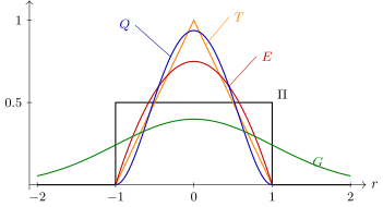
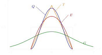
Frequently used kernels: , Epanechnikov; , quartic; , triangular; , Gaussian; , rectangular.
Definition (The choice of kernel).
- , the optimal one (Epanechnikov);
- , quartic;
- , triangular;
- , Gaussian;
- , rectangular.
Which kernel to choose? The piecewise-constant, rectangular kernel is an unfortunate choice, because the density estimate will come out piecewise-constant. And all the others are approximations, including smooth ones, such as the Gaussian. What is wrong with the Gaussian? It takes into account all the objects of the sample; it is not a localised density. And what if we take, for example, the quartic kernel, a piece of a fourth-degree polynomial on the segment ? What is good about it: first, the function is smooth, even at zero, unlike the piece of a parabola, which is continuous but not smooth at the ends of the segment; and second, it is finite: only on the segment is it non-zero, and outside it it equals zero. The quartic kernel is a very frequent choice; it really is often used.
Proposition. The functional of the quality of density estimation:
The asymptotic values of the ratio as do not depend on the form of the distribution :
| Kernel | Degree of smoothness | |
|---|---|---|
| Epanechnikov | discontinuous | 1.000 |
| Quartic | discontinuous | 0.995 |
| Triangular | discontinuous | 0.989 |
| Gaussian | differentiable | 0.961 |
| Rectangular | discontinuous | 0.943 |
The choice of kernel has almost no effect on the quality of estimation.
There are theoretical results showing that in fact the choice of kernel has almost no effect on the quality of density estimation, but it does, of course, affect the smoothness of the resulting density. I will not dwell long on this result: practically all kernels give a value of the quality criterion very close to the optimal one, and the optimal one, strangely enough, is given by a piece of a parabola that is called the Epanechnikov kernel. On the other hand, the criterion raises questions: why do we compare densities in effect by the method of least squares? That is not a very good thing to do, but as for why, let us leave it for now; I will tell you some day.
The choice of window width
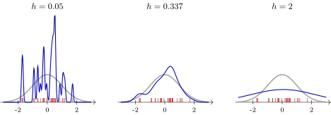
The Parzen–Rosenblatt estimate with a Gaussian kernel on one and the same sample of 30 points from the standard normal distribution (red ticks) for three values of the window width (a schematic after the slide; the sample is generated). The grey curve is the true density. With the estimate jerks after every point (overfitting), with it is heavily smoothed out (underfitting), and is the optimal width in the example on the slide.
But the width of the smoothing window is precisely the parameter on which the quality of density estimation depends critically. The smoothness of the density estimate depends on the kernel, and its quality on the window width. On the slide there is an example: the sample is one-dimensional, blue points on the horizontal axis, clearly Gaussian; in grey the graph shows the true density, a Gaussian with zero expectation and unit variance. We try to recover it with different window widths. With the optimal window width we get a more or less decent approximation: the black curve is similar to the grey one. Take the window too small, and the estimate starts jerking after every point of the sample; these little spikes, these outliers arise because the density comes out too heavily jagged. This is overfitting: we start fitting to particular data points. And if we take too large, there will be underfitting; as tends to plus infinity, the estimate is smoothed out and tends to a uniform distribution. There is always a golden mean between the extreme cases: a window that is too small gives a noisy, overfitted model; one that is too large gives a model that does not describe the features of the data.
Definition (The choice of window width).
- The quality of density estimation depends essentially on the window width , but weakly on the form of the kernel .
- When local concentrations of density are inhomogeneous, one can set , where is the number of neighbours.
- Leave-One-Out cross-validation for density estimation by maximum likelihood:
The typical form of the dependence (slide): for small , overfitting; for large ones, underfitting; the optimal window width is in the neighbourhood of the minimum.
This is probably the main understanding: in Parzen density estimates it is very important to choose the window width; the quality of density estimation depends critically on it, and not much on the form of the kernel. The window width is very often chosen by leave-one-out: we train on the whole sample except one single point, and at that point we look at the loss function, the log-likelihood with a minus sign. Remember: the maximum likelihood principle maximises, so if we minimise, we must put a minus in front of the logarithm. We get a dependence with a minimum: on the left, for small , overfitting; on the right, for large ones, underfitting. We look for the neighbourhood of the minimum and say: here we have determined the optimal window width. That is what is done most often.
A retrospective: three problems with one construction
Definition (A retrospective: (non)parametric, a.k.a. metric, methods of data analysis). Density estimation. The Parzen–Rosenblatt method:
Classification. The Parzen window method:
Regression. The Nadaraya–Watson kernel smoothing method:
This is very similar to what we have already seen when we considered the Parzen window method for metric classification algorithms and the method of nonparametric regression, the Nadaraya–Watson formula. Let us look at them all together and realise what we have just done. What is a nonparametric density estimate? It is a metric method. "Nonparametric" and "metric" are a play on words: they seem to be different things. "Nonparametric" means that we do not use a parametric model, and "metric" that we use a distance function between objects. At first sight these are quite unrelated things, but here they almost coincide, and it is correct to use either name.
We looked at the Parzen window method as a heuristic generalising the nearest neighbour method, and at its basis lay the distance between objects. Then we saw nonparametric regression methods, the Nadaraya–Watson kernel smoothing formula, and there too everything is based on the distance function between objects. And now we have realised that density estimation is the same kind of thing. All three problems have one common construction: a kernel and the choice of the width of the smoothing window in this kernel. The choice of kernel determines the smoothness of the function, whatever it is, a regression dependence, a separating surface in a classification problem or a density function, and the accuracy of the approximation is determined by the window width. This undoubtedly unites all three problems. The problems are different: classification and regression are supervised learning, density is unsupervised learning, but the approaches are very similar.
Three approaches to density estimation
Between the parametric approach, the nonparametric one and the separation of a mixture of distributions there is also an interesting fundamental connection. Look: nonparametric density estimation is in effect a mixture of distributions, with a distribution of its own at each data point. What is a kernel? It is a density in itself, and we have added up such densities. So this is a mixture, and with equal weights at that: each point, each object, has generated its own mixture component of some not very large width, and together in the mixture they have formed the density estimate.
You asked how to determine the optimal number of mixture components. And here I am showing that they can even be set equal to the number of objects of the training sample. True, such a thing cannot be tuned by the EM algorithm: there would be very heavy overfitting; a sample of objects cannot be described by mixture components. But here it turned out that it can: for each data point we built a mixture component of its own, with this point at its centre. This is a very extreme special case of a mixture, where the number of components is chosen not at all optimally, but since we fixed the window width, it does not lead to bad consequences such as overfitting, and the window width can be chosen for all mixture components at once. They are all of the same shape and width, and each is placed at its own object of the sample.
- parametric: , ;
- mixture separation: , ;
- nonparametric: , .
It turns out that recovering a mixture of distributions is, one might say, the golden mean between the ordinary parametric approach, which is a mixture of one component, and the nonparametric one, which is a mixture of components, where is the number of objects in the sample. And a mixture of components, if is determined optimally, is the most balanced approach: it is more general than both the parametric and the nonparametric one. That is an interpretation of how these three approaches to estimating probability densities are positioned: the mixture is probably the most general thing there can be.
Bayesian classification theory
Now let us take up classification; this is the second half of the lecture, though literally twenty minutes or so are left for it. Look what a very simple idea: if, when solving a classification problem, we learned to recover the density of each class, could we, knowing the estimates of the class densities, easily build a classifier? The answer is yes. This is called Bayesian classification theory: reducing the classification problem to the problem of recovering the distribution in each class separately.
Generative models of classification
Definition (Probabilistic generative models of classification). are the objects, the classes, a probability space with density .
Given: a simple sample .
Find: a classification model .
Criterion: minimise the probability of error .
Suppose the joint density is known:
- is the prior probability of the class ;
- is the likelihood function (density) of the class ;
- is the posterior probability of the class .
By Bayes' formula .
The Bayes classifier:
Let us begin with the formulation. Now the objects are distributed over classes, and we consider that the joint space of "object–answer" pairs is a probability space with an unknown joint density of objects and answers, and our simple, i.i.d. sample came from this density. We are required to build an optimal classifier. Let us suppose for now that the joint density is known; later, of course, we will estimate it from the sample. If it were known, we would write it out by the formula for conditional density, or conditional probability, in two ways.
Let us look carefully at these expressions; here it is important not to get confused and to remember once and for all what is what, because this approach is used in many other places in machine learning. Of the four quantities, these are the ones we will need. The first is the prior probability of a class: what share of the objects of the sample lies in each class at all. Prior probabilities we can estimate by frequencies, the share of the sample in the class . Next is the likelihood function of a class. What kind of beast is that? If we look at the class , it is the density that the objects of this class have. This is exactly what we can recover as a density from the training sample: we take only the objects of the class and recover the density from them, which we have just learned to do. And the last, , is the posterior probability of a class: a posteriori because it appears after we have been given a fixed object and asked which class this could belong to. By Bayes' formula it is this thing.
Excellent. To which class, then, should the object be assigned? To the one whose posterior probability is maximal. The construction appears. But note: the is taken over the classes , and the denominator does not depend on . It does not even need to be estimated; it can simply be thrown out: under the over it is just a constant. The joint density of all in all classes can be computed, but we simply do not need it. We need to estimate the prior probabilities of the classes and the densities of the objects in each of the classes, and this gives the Bayes classifier, so called because it is built by Bayes' formula.
Definition (The Bayes classifier and maximum likelihood). Given: a simple sample .
Find: the parameters of the model .
Criterion: the maximum likelihood method:
where are all the objects of the class in the sample .
Decomposition into independently solved subproblems:
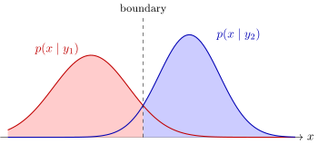
Classification by the maximum of the likelihood function when the prior probabilities of the classes are equal: an object is assigned to the class whose density is larger at the given point; the boundary between the classes runs where the densities intersect (a schematic).
An illustration: if the prior probabilities were equal, the classification rule would become quite simple. At each object that we want to classify, we have to compute the density estimates for each of the classes and assign to the class for which the density estimate is maximal. Two classes, each described by its own density, and they have intersected; it seems that the intersection is the boundary between the classes, and we will need this consideration again. In one region one class has the larger density, in the other the other. A very simple visual interpretation of the Bayes classifier.
The discriminative and generative approaches
Definition (Two approaches to learning classification).
- Discriminative: are non-random vectors; is a classification model. Examples: LR, GLM, SVM, RBF.
- Generative: are random vectors; is a model of data generation. Examples: NB, PW, FLD, RBF.
Bayesian classification models are generative:
- they model the shape of the classes not only along the boundary but over the whole space, which is excessive for classification;
- they need more data to train;
- but they are more robust to noise near the class boundary.
This is in fact a very deep consideration about how to solve classification problems in general: whether to build a separating surface or to recover the probability densities of the classes. It is a very serious dichotomy in classification methods, and the approaches are called discriminative and generative. The discriminative one says: at each object we will recover only the posterior probability, estimate with what probability the object belongs to a class. For this one can use, for example, a geometric approach: we build some separating surface, and the objects that turn out to be far from it belong to their class with high probability. This is like the support vector machine, which really is based on geometric assumptions; or logistic regression, where the posterior probability of the classes is modelled explicitly through a linear separating surface. The other approach is generative: we want to understand which densities the objects came to us from, to build density models for each class. This is in effect a model of data generation: each class had its own generating density, and we want to find out which. There are quite a lot of such examples too: for example, Parzen Window, the Parzen window method, or radial basis functions; the other abbreviations we do not know yet.
Which of the approaches is better cannot be said: sometimes one, sometimes the other, depending on the situation. But in the generative approach we are clearly doing some extra work: we try to describe the densities of the classes, including the objects that lie far from the separating surface. Why, one asks? We need only the classification, only the separating surface, which means the densities need to be described at the boundary between the classes, while we try to describe them entirely, over the whole space. It seems that we are doing extra work and hunting for peripheral objects that do not affect the quality of classification. That is why generative models need more data to train. But at the same time, since we recover the density, then, if the density model is decent, it will allow outliers to be ignored better: the robustness to noise is greater. When we discussed SVM, we said that the support objects turn out to be not only the objects on the boundary but also the objects that have jumped over the boundary, have become outliers, lie in another class, and we still use them as support objects. That is probably not very good. A generative model would tell us that these are objects at which the value of the density is very small, close to zero, so they can and should be ignored. There are many attempts to combine the merits of the discriminative and generative theories of classification.
The optimal Bayes classifier
Theorem (The optimal Bayes classifier). Let and be known, and let be the loss from an error on an object of the class . Then the minimum of the average risk
is attained by the optimal Bayes classifier
Remark 1: after the empirical estimates and are substituted, the Bayes classifier is no longer optimal.
Remark 2: the problem of estimating a probability density is harder than the classification problem.
I do not prove the theorem on the optimality of the Bayes classifier in this course; it is proved in the course of mathematical statistics and is not at all difficult. It says: if we knew the prior probabilities and the likelihood functions of the classes, that is, the class densities, we would write out the method of minimising the average risk, this functional, and the theorem states that the classifier for this must be built like this, as the of this expression. What we realised intuitively, on our fingers, is in fact the theorem on the optimality of the Bayes classifier.
The only thing we did not talk about then is , the losses from errors. We minimise the average risk, the expectation of the losses, where the size of the loss is , and it enters the optimal Bayes classifier as a factor. This is the only thing we could not have guessed intuitively. If you introduce a cost of error on the objects of the class and this cost, for example, has doubled, it is the same as if the probability of objects of this class appearing had doubled. That is, and form a product; is in some sense a recalculated estimate of how often objects of this class will appear for you; they flow into each other. That is why in Bayesian classification theory the product is always considered from here on.
And one more sardonic remark: of course it is not optimal at all; "the optimal Bayes classifier" is only a name. It is optimal only if the class densities are known exactly. As soon as we start estimating them from the sample, there can be no talk of any optimality: sample estimates of probability densities may well be overfitted. The Bayes classifier with estimates substituted into it is simply a way of constructing classifiers on the basis of a probabilistic model of the classes, nothing more.
And it seems that this is a bit of using a sledgehammer to crack a nut, because estimating densities is, generally speaking, a harder problem than classification. Why? Densities are estimated in a function space, a density is a continuous function, while in a classification problem there is a finite number of classes; classification is a piecewise-constant function, and recovering it seems simpler. Although both are recovering a function from data, so perhaps one cannot judge unambiguously that we are reducing the simpler classification problem to solving the harder problem of density estimation. People sometimes say so, but it is an interpretation, not a strict mathematical fact.
A survey of Bayesian classifiers
I will skip the piece about the naive Bayes classifier, although it is of course interesting, and go straight to the survey. We have to substitute density estimates into the construction of the optimal Bayes classifier, and today we have learned three types of them: parametric, nonparametric and mixtures of distributions. Let us do it.
The Parzen window method
Definition (The Parzen window method (Parzen Window, PW)). The nonparametric Parzen–Rosenblatt density estimate with a distance function for each class :
The Parzen window method is a metric classifier:
Remark 1: the normalising factor cancels under the if it does not depend on and .
Remark 2: the problems of choosing the kernel , the window width and the distance function remain.
Let us begin with the simplest case. If we substitute the nonparametric density estimate into the optimal classifier, we unexpectedly discover the Parzen window method, which we have already covered, a metric classifier; that is just how we wrote it out. The only thing we did not have then is the factor . It may cancel if the number of objects in a class is proportional to the prior probability of the class, that is, if there was no special distortion when the data were formed. But if, for example, the classes were unbalanced and you balanced them, evened them out, then this balance must be taken into account, in exactly this way. In the metric classifier there was no talk of this, so we did not know that such a factor had to be put in there too. It turns out that the Parzen window method, which we derived as a heuristic generalising the nearest neighbour method, is in fact statistically justified: it is the optimal Bayes classifier with the Parzen–Rosenblatt density estimate substituted into it. Such is the connection that has formed between two approaches that at first sight are about completely different things.
Remark (The window width in classification and in density estimation). In the Parzen density estimate there is a dreadful normalising factor , an integral that one has to be able to compute, and that is, generally speaking, non-trivial. But in the Parzen window method it is absent. Why? Because it has cancelled. This is rarely written anywhere: one has to contrive to estimate the class densities so that at each point the window width is the same for the different classes; otherwise one would have to put in normalising factors of their own for the different classes. Being at the point and trying to classify this object, we must use the same window width in the density estimates for all classes. At this point there may be many of some class and none at all of another, whose density is small here, and there is a temptation to use for each class its own density estimate with a variable window width: where the objects of a class are dense, make the window smaller, and where they are sparse, larger. Well, in the Parzen window method this must not be done. If you are estimating a density, it should be done: there turned out to be zero objects in a narrow neighbourhood, you have landed at a point of sparsity, and to recover the density a variable window width is needed. But if you are solving a classification problem, you categorically do not need to do this: at each point the density must be estimated for all classes with a single window width. Such is the little subtlety.
The quadratic discriminant
What if we apply the parametric approach, if the class densities are Gaussian? This leads to an interesting construction called discriminant analysis. It was studied a great deal from about the thirties to the sixties. Nowadays discriminant analysis is practically not used, because logistic regression and SVM certainly work better, but for general education it is good to know what it is.
Theorem (The quadratic discriminant (Quadratic Discriminant Analysis)). The hypothesis: each class has an -dimensional Gaussian density with centre and covariance matrix :
- The separating surface defined by the equation is quadratic for all .
- If , the surface degenerates into a linear one.
The quadratic discriminant is a plug-in algorithm:
An interesting point: if the densities are Gaussian, what will the separating surface look like? It is the locus of points where the expressions under the for two classes are equal. If we take logarithms, we get the first statement: the separating surface is quadratic. The quadratic form enters only in the construction with the inverse covariance matrix. If the covariance matrices of the Gaussian classes are the same, and that means the classes are of the same shape, their scatter ellipsoids are, as it were, moved apart by a parallel translation, identically oriented and with identical variances, then the quadratic terms cancel, and the separating surface degenerates into a linear one. This construction is called the linear discriminant, Fisher's linear discriminant: a linear separating surface, even if the classes are not spherical, as long as they are of the same shape, with the same covariance matrices.
On the slide there are six pictures with the geometric meaning of the quadratic discriminant. When we play with the factor , the separating surface simply shifts in parallel. The rule is easy to remember: it moves away from the most dangerous class, the one that either appears more often or has a larger , the loss from an error on objects of this class. If the classes are of different shapes, the surface is quadratic, and it can be so quadratic that a strange situation arises: a point that lies far away, closer to the objects of the other class, you will suddenly assign to the first class. This is an artefact of the method, an artefact of the generative approach: you estimate densities and then use them for classification, and far from the boundary between the classes anything can happen; the density estimate there may simply be inadequate, and for both classes at that. And situations where the classes are dissolved in each other are another matter: nothing can be done there; that is an unsolvable classification problem.
Fisher's linear discriminant
Theorem (Fisher's linear discriminant (Fisher Linear Discriminant)). The problem: for classes with few objects, is possible.
Let the covariance matrices of the classes be equal: , . The maximum likelihood estimate for :
The linear discriminant is a plug-in algorithm:
In the case of multicollinearity, invert the matrix .
A little more about Fisher's linear discriminant. When you have described all the classes by densities with one and the same covariance matrix, you determine the estimate of this matrix, by and large, from the whole sample: the shape of the classes is the same, so it should be estimated from the full sample, only you shift each object by the expectation of its class . Such is the small correction to how the covariance matrix then has to be estimated. It is as if you determined the centre for each class, brought the centres together at one point by a parallel translation, so that all the objects have shifted, and estimated the common covariance matrix from this sample.
The classifier comes out linear. To estimate it, one has to be able not only to compute the covariance matrix from the data but also to compute its inverse. Then by these formulas we compute the free terms and the coefficients of the linear classifier . For each class we get a linear function of its own, and the direction vector of the -th class says in which direction the objects of this class lie: the farther in that direction, the more numerous and denser the objects of this class will be. Here is one more geometric interpretation: for each class you have indicated the direction in which its objects are predominantly located. Clearly, the thing is not ideal. But it is one more example of a linear classifier. How many do we have already: SVM is one, logistic regression two, Fisher's linear discriminant three, and if you scrape around, a few more will be found in our course; many times we have recalled linear classifiers.
Remark (The geometric interpretation of the linear discriminant). In the one-dimensional projection onto the direction vector of the separating hyperplane, the classes are separated in the best way, that is, with the minimal probability of error; the projection axis is perpendicular to the common tangent of the scatter ellipsoids.
Ronald Fisher, a statistician after whom a great many things in statistics are named, came up with this in 1936. This is the very same Fisher of the irises: remember, three classes. He described them precisely by Gaussians and then came up with a principle for separating clusters of points optimally: let us describe them by Gaussians and see in which direction these Gaussians project onto a one-dimensional axis so well that they separate as sharply as possible. The sharpness of separation is the minimum of the overlap of the one-dimensional Gaussians: a multivariate Gaussian density, if projected onto an axis, becomes a one-dimensional Gaussian. Fisher was solving the problem of how to minimise the overlap of these Gaussians and, unexpectedly, discovered the optimal Bayes classifier. We obtained it from much more general considerations, and the optimality there is a theorem valid for any densities, while Fisher in 1936 derived it exclusively for Gaussian ones. For us this is rather of historical interest: practically nobody uses Fisher's linear discriminant any more, although in the sixties it was mainly what was used; SVM was not yet known.
Fisher R. A. The use of multiple measurements in taxonomic problems, 1936.
Gaussian mixtures and the radial basis function network
The last story I wanted to tell. Two stories I actually did not get to: about the naive Bayes classifier and about the Gaussian mixture with diagonal covariance matrices. Let us describe each class in the optimal Bayes classifier by a Gaussian mixture; I will show right away where we will end up.
Definition (The radial basis function network (RBF)). Let the likelihood functions of the classes be representable as mixtures of Gaussian components with uncorrelated features for each class :
In the multiclass classification problem, , the EM algorithm trains a three-layer RBF network:
The radial basis function network (slide): the first layer computes the densities of the mixture components of each class, the second mixes them with the weights , the third chooses the class by ; this is the optimal Bayes classifier.
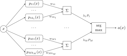
The radial basis function network: the first layer computes the densities of the mixture components of each class, the second mixes them with the weights , the third chooses the class by ; this is the optimal Bayes classifier.
We take all these estimates, which of course are obtained by the EM algorithm, substitute them, and unexpectedly discover an interesting construction called the radial basis function network, a three-layer network. The first layer computes the estimates of the mixture components for each class, the second layer mixes the components, and the third is the , the optimal Bayes classifier. The density of each class is described by components, and each class may have its own number of components . In architecture this is RBF, radial basis functions, and such a network is trained by the EM algorithm: for each class separately you recover a mixture of distributions by the EM algorithm. The number of components can be chosen there, which is the number of neurons in the first layer for each class, roughly as I described: increase it a little, decrease it a little.
Remark (An RBF network trained by the EM algorithm, and SVM with a Gaussian kernel). Remember RBF? It is arising for us for the third time in the course. Last time we talked about SVM: SVM with Gaussian kernels also leads to such a construction, but there, oh joy, the number of components, which here is generally non-trivial to choose, was simply the number of support objects and came out of the SVM method automatically. The architecture is one and the same, but the training methods are very different. And the first time it arose was when we talked about the method of potential functions: constructions of this kind arose there too, and then too we called it a radial basis function network.
How the generative RBF-EM differs from the discriminative RBF-SVM:
- the support vectors are not boundary objects of the sample but the centres of local concentrations of the classes;
- a structural description of each class as a set of components, clusters, is built automatically.
Advantages of the EM algorithm: it is more robust to noise outliers and, as a rule, converges fairly quickly.
Drawbacks of the EM algorithm: it is sensitive to the initial approximation; determining the number of components is a hard problem (simple heuristics may work poorly).
Where this is applied
Is this applied now? Strangely enough, it is. Mixtures of distributions arise often and in many places. Should mixtures of distributions be used to recover classes in a classification problem? Sometimes they should: when we want to understand the internal structure of a class. There is a more general approach that really is applied: solving a classification problem through a clustering problem. First we understand the internal structure of each class, and this allows the classification problem to be solved more accurately. Gaussian mixtures for the optimal Bayes classifier are sometimes used precisely when something more than just classification is needed.
The second case is that very naive Bayes classifier that I did not have time to tell about. It is often used as a whipping boy, as a baseline: very simple, very easy to train, but it is a feeble classifier, based on the draconian assumption that the features are independent, so it rarely works anywhere. But sometimes it does work, for example in text analysis, where the features are word frequencies: there are very many words, and to a first approximation they can be considered independent of one another, so there the assumption can be stretched to fit, more or less.
In general, Bayesian classification theory is an achievement of somewhere around the sixties and seventies, and it still works in many places, wherever we need a generative approach. It may be needed for various reasons: it is not necessarily a strong classifier, but it does recognise the internal structure of the classes. Sometimes one needs to split a class into components and also estimate the probabilities of an object belonging to these components, that is, the reason why this object ended up in this class. Sometimes such things are needed for estimating risks, for obtaining structural information about what kind of object this was.
Conclusions
Density estimation from a sample, three approaches: parametric (), mixture separation (), nonparametric ().
Probabilistic models of classification, two approaches, both based on maximising the likelihood:
- discriminative: we model , are not random;
- generative: we model for all ; more demanding of the amount of training data, less sensitive to noise outliers.
Bayesian classification theory:
- the main formula: ;
- the naive Bayes classifier is based on the assumption that the features are independent.
No comments yet
Be the first to share your thoughts.