August 30, 2026 · Lecture · LibreTimes
Machine Learning 1. Lecture 14. Anomaly Detection and Robust Methods
Contents
- What this lecture is about
- Detecting anomalous objects
- Anomaly detection problems
- Heuristics for scoring anomaly
- Removing outliers in nonparametric regression
- Putting the approaches together
- The theory of robust learning
- Slowly growing functions
- Iterative reweighting of objects
- Robust loss functions
- Robust aggregation functions
- Iterative reweighting for an aggregation function
- Examples
- Problems with anomalous or new classes
- One-class classification
- Learning from a sample of one class
- Problems with new or unknown classes
- Summary
What this lecture is about
Training data are almost never clean: they contain measurement errors, typos, objects the model describes poorly, and objects unlike anything seen before. The lecture has three parts. The first covers the problems of detecting anomalous objects and simple heuristics for scoring anomaly. The second is the theory of robust, that is, noise-resistant, learning: robust loss functions, robust aggregation functions and methods of iterative reweighting of objects, which make it possible to train a model so that outliers hardly affect it. The third covers problems with anomalous or new classes: one-class classification, learning from a sample of a single class, and problems in which the set of classes is not fixed in advance.
Detecting anomalous objects
Anomaly detection problems
Definition (Anomaly detection problems). Outlier detection:
- errors in the data of a training or test object;
- the model is inadequate on some objects.
Novelty detection:
- nothing like it was in the training sample.
Applications:
- fraud detection;
- intrusion detection;
- detecting insider trading on an exchange;
- detecting faults from sensor readings;
- medical diagnosis.
Two settings are distinguished. An outlier is an object of the training or test sample that does not fit the general pattern: either its data contain an error, or the model is inadequate on it. Novelty is an object unlike anything in the training sample. In detecting fraud, intrusions into computer networks or equipment faults, the anomalous objects are precisely what is of main interest; in training models, on the contrary, they get in the way, and one wants to find and neutralise them.
Heuristics for scoring anomaly
Most methods assign each object a number, its anomaly score: the larger it is, the less the object resembles the others. There are many ways to define such a number, and each rests on its own idea of how normal data are arranged.
Definition (The metric approach (Breunig, Kriegel, Ng, Sander, 2000)). The anomaly score of an object is the distance to its -th nearest neighbour: the larger it is, the lower the local density of the sample.
M. M. Breunig, H.-P. Kriegel, R. T. Ng, J. Sander. LOF: identifying density-based local outliers. 2000.
If there are few other objects around an object, the distance to its -th neighbour is large, and the object lies in a region of low density. This is the same principle as in the nearest neighbours method and in Parzen density estimates, except that what is estimated is the density, not the class.
Definition (Random isolation forest (Isolation Forest; Liu, Ting, Zhou, 2008)).
- A random forest of trees is built.
- Each split: a random feature and a random threshold.
- Each leaf holds only one object.
- The anomaly score of an object is the mean depth of the leaves it falls into: the smaller it is, the more isolated the object.
Fei Tony Liu, Kai Ming Ting, Zhi-Hua Zhou. Isolation Forest. 2008.
The idea of the isolation forest: random splits quickly separate an object lying far from the others — a few thresholds suffice — while an object in the thick of the sample takes a long time to isolate. So a small mean leaf depth indicates an anomaly. The trees are built without any quality criterion, which makes the method very fast.
Definition (Separating a mixture of distributions with a background component). The generative model of a mixture of distributions:
Ways to specify the background distribution :
- a spherical Gaussian with a large variance;
- a radial distribution with a heavy tail (Laplace, Student's ).
The problem of maximising the log-likelihood:
The anomaly score of an object is the probability that it belongs to the background; it is estimated at the E-step of the EM algorithm.
This generalises the mixture of distributions that was solved by the EM algorithm in the lecture on density estimation. One more component is added to the usual ones, a wide "background" one, which has to describe everything the others do not. The E-step itself computes the posterior probability that the object was generated by the background, and that is its anomaly score.
Definition (Robust principal component analysis (Robust PCA; Candès, Li, Ma, Wright, 2009)). are the original numerical features of an object ; are new numerical features, ;
is the reconstruction of the old features from the new ones.
Find both the new features and the transformation at once:
The anomaly score of an object is an unknown sparse noise :
where is a low-rank matrix and is a sparse matrix.
Principal component analysis approximates the object–feature matrix by a low-rank matrix. If the data contain isolated corrupted values, ordinary principal component analysis tries to explain them too, and is distorted. The robust variant allows part of the data not to be explained by the model: the residual is collected in the matrix , and the penalty makes it sparse. The nonzero entries of show which objects, and which of their features, are anomalous.
Removing outliers in nonparametric regression
Recall kernel smoothing from the lecture on metric methods.
Definition (Reminder. Nonparametric regression). The regression model is a constant in a neighbourhood of :
where are the weights of the objects relative to ; is a kernel, non-increasing, bounded and smooth; is the width of the smoothing window.
The Nadaraya–Watson kernel smoothing formula:
The Nadaraya–Watson estimate is a weighted mean of the responses of neighbouring objects. The mean is unstable under large outliers: one object with a huge distorts the estimate throughout its neighbourhood. The natural idea is to reduce the weights of the objects on which the error is large. But the error can only be estimated by building a model, and the model depends on the weights. There is no vicious circle here: it is a reason for an iterative process.
Definition (The LOWESS algorithm (LOcally WEighted Scatter plot Smoothing)). Input: , the training sample. Output: coefficients , .
- initialisation: , ;
- repeat
- leave-one-out estimates at each object:
- , ;
- until the coefficients stabilise.
Gary W. Moran. Locally-Weighted-Regression Scatter-Plot Smoothing (LOWESS): a graphical exploratory data analysis technique. 1984.
At each iteration, for each object, an estimate of its response is built from all the other objects — a leave-one-out estimate in which the object itself takes no part, otherwise an outlier would "explain" itself. The error is converted into the object's weight by one more kernel : the larger the error, the smaller the weight with which the object enters the estimates for its neighbours. The kernel can be chosen in different ways. Hard filtering: build the order statistics of the errors and discard the objects with the largest error, which corresponds to . Soft filtering: take the quartic kernel with a width proportional to the median error, .
LOWESS on synthetic data (slide): , , Gaussian kernel ; two of the 100 points are outliers with ordinates and (off the plot). The pale curve is the Nadaraya–Watson estimate without reweighting, distorted by the outliers; here LOWESS converges in a few iterations.
The example shows how badly two outliers spoil ordinary kernel smoothing: each of them pulls the curve towards itself over a distance of the order of the window width. After a few LOWESS iterations their weights become practically zero, and the curve follows the bulk of the points.
Putting the approaches together
Definition (Reminder: the least absolute deviations method). A loss function , where is the error; is the criterion for training the model on the sample.
The least squares method, :
The least absolute deviations method, :
where are the order statistics of the values . The median is more robust to rare large outliers .
The simplest model, a constant, shows the essence of the matter. The minimum of the sum of squares gives the mean, and a single object with a huge shifts it arbitrarily far. The minimum of the sum of absolute values gives the median, which does not depend on the size of an outlier at all, as long as fewer than half of the objects are outliers.
Definition (Reminder: SVM regression is also robust regression). The regression model: , , . The loss function is piecewise linear: .
The problem:
The problem is solved by a change of variables and a reduction to a quadratic programming problem.
The SVM regression loss grows linearly rather than quadratically, so it too is insensitive to large errors, in the same sense as the least absolute deviations method.
Definition (Novelty detection and other problems). The anomaly score of an object (anomaly / novelty / surprise score) is the value of the loss function on that object.
Ways of scoring anomaly:
- the anomaly is scored for an object of the training sample (outlier) or for a new object (novelty);
- the loss depends on (supervised) or not (unsupervised);
- when the anomaly of a training object is scored, the object is excluded from the sample, , or not, ;
- the loss function is the same as in the training criterion, or not.
Ways of using anomaly scores:
- hard removal of anomalous objects from the sample;
- soft reweighting of objects.
M. Salehi et al. A unified survey on anomaly, novelty, open-set, and out-of-distribution detection: solutions and future challenges. 2021.
All the heuristics considered fit one scheme: the anomaly score is the model's loss on the object. In the metric approach the model is the local density, in the mixture it is the likelihood, in robust PCA the reconstruction error, in LOWESS the leave-one-out error. The schemes differ in whether there are responses , whether the object itself takes part in training the model by which its anomaly is scored, and in what is done with the anomalies found: they are removed, or their weights are reduced.
The theory of robust learning
Slowly growing functions
Definition (Optimisation problems of machine learning). The problems of regression, classification, clustering, density estimation, dimensionality reduction and others differ in their loss functions and regularisers :
The problem: outliers can distort and the criterion .
The idea: reduce the weight of outliers with large by introducing slowly growing functions :
Almost all the learning problems in the course have this form: a sum of losses over objects plus a regulariser. If the loss on an outlier is large, that object determines the solution. A slowly growing function "flattens" large losses. The condition for an extremum shows that this is equivalent to weighting the objects: each object enters the gradient with weight , and if decreases, objects with large losses get small weights.
Iterative reweighting of objects
Definition (Iterative Reweighting Scheme (IRS)). Let be a slowly growing function: , , decreases, as .
Input: , the loss function on the training sample. Output: the model parameters , the object weights .
- initialisation: , ;
- repeat
- ;
- , ;
- until the weights stabilise;
where is the normalisation of a vector.
Drawback: everything goes badly when the outliers are large or numerous.
The condition for an extremum cannot be solved at once, because the weights depend on . But if the weights are fixed, what remains is an ordinary learning problem with weighted objects, which we know how to solve. Hence the iterative scheme: train the model with the current weights, recompute the weights from the losses, repeat. This is the same device as in LOWESS, only in general form, for any model and any loss function.
Definition (Iteratively Reweighted Least Squares (IRLS)). Robust regression: .
Input: , the training sample. Output: the model parameters , the object weights .
- initialisation: , ;
- repeat
- ;
- , ;
- until the weights stabilise.
Drawback: everything goes badly when the outliers are large or numerous.
In regression it is more convenient for each iteration to solve a least squares problem, for which fast methods exist. To that end the loss is written through the squared error: , and . So the weight of an object in the least squares problem is . With this gives the least absolute deviations method, solved by a sequence of weighted least squares problems with weights .
Robust loss functions
Definition (Loss functions for robust regression). The loss is a function of the error . The quadratic loss is not robust.
Robust loss functions with a parameter :
- — piecewise linear (Least Absolute Regression);
- — piecewise linear (SVM Regression);
- — Meshalkin's;
- — Huber's;
- — Tukey's;
- — Andrews'.
Barron's family of functions with a parameter :
Jonathan T. Barron. A General and Adaptive Robust Loss Function. 2019.
Robust loss functions are of two types. In some the branches grow linearly (absolute value, SVM regression, Huber): large errors are taken into account, but not as strongly as with a square. In others the branches approach a horizontal asymptote or become constant (Meshalkin, Tukey, Andrews): beyond some size of error the object stops affecting the solution altogether. Huber's function is a compromise: near zero it is quadratic and smooth, and further out it is linear.
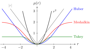
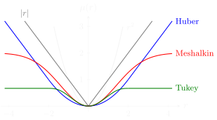
The quadratic loss (black) and robust ones: absolute value (grey), Huber's (blue), Meshalkin's (red), Tukey's (green), all with .
Barron's family brings many of these functions under one parametrisation. At (as a limit) it gives the quadratic function , at a smooth analogue of the absolute value , at (as a limit) the logarithmic function , and as a function with a horizontal asymptote, , which up to scale is Meshalkin's function. By decreasing one can continuously change the model's attitude to large errors, from full trust in the data to ignoring them; the parameter can even be tuned together with the model.
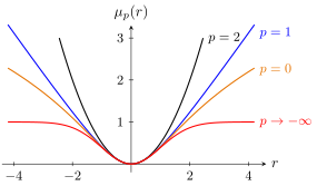
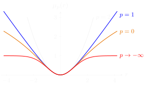
Barron's functions for , , and (the values at and are limits of the formula). The smaller , the more slowly the branches grow.
Experiments with robust regression on synthetic data show a typical picture. While there are no outliers, all loss functions give almost the same lines. With 10% outliers the quadratic loss already distorts the solution noticeably, while Huber's does not. With 30% and 50% outliers the robust loss functions, Huber's and Tukey's, give in too: the line turns towards the outliers. The iterative reweighting scheme works poorly when the outliers are large or numerous.
Robust aggregation functions
Another view of the same problem: the training criterion is a sum, that is, up to a factor, the arithmetic mean of the losses over the objects. And the arithmetic mean is the least stable way of aggregating. It can be replaced by a stable one.
Definition (Robust (outlier-resistant) ways of averaging). The arithmetic mean (not robust to large outliers):
Robust ways of averaging, defined through the order statistics of the values :
- the median:
- the -quantile:
- the censored mean: .
Drawback: these averaging functions are not differentiable.
The median of the losses, their quantile or their censored mean (large losses are replaced by the -th largest value) hardly react to a few huge values. But if we substitute the losses and minimise such an aggregation function over the model parameters, we run into non-differentiability: the order statistics rearrange in jumps as changes. The way out lies in two ideas.
Definition (The general form and properties of aggregation functions). Idea 1: replace the mean by a one-dimensional minimisation over .
Idea 2: then replace the absolute value by a smooth approximation of it.
Properties of the dissimilarity function : strictly convex, , .
Properties of the aggregation function :
- ;
- monotonicity: ;
- symmetry: for any permutation ;
- Cauchy mean: .
All three ways of averaging — and the arithmetic mean itself — are written as the solution of a one-dimensional problem: find the point least dissimilar to all the . The squared dissimilarity gives the mean, the absolute value the median, the asymmetric absolute value the quantile. It remains to replace the absolute value by a smooth strictly convex function, and the aggregation function becomes smooth in its arguments.
Definition (Examples of smoothed dissimilarity functions). The smoothed absolute value (to approximate the median):
The smoothed asymmetric absolute value (for the -quantile):
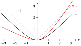
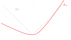
The smoothed absolute value with (black) next to the absolute value (dashed), and the smoothed asymmetric absolute value with (red): to the right of zero the branch is multiplied by , to the left by .
Definition (One more example: the smoothed censored mean). We use the identity :
The censored mean is smoothed in two steps: the threshold is replaced by the smoothed -quantile , and the minimum of two numbers is expressed through the absolute value, which is also replaced by a smoothed one.
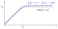
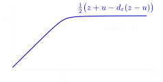
The function (dashed) and its smooth approximation with .
Iterative reweighting for an aggregation function
Now empirical risk minimisation can be generalised: what is minimised is not the sum of the losses but an aggregation function of them.
Definition (Generalised empirical risk minimisation (ERM)).
The iterative reweighting algorithm (IR-ERM):
- repeat
- ;
- , ;
- until the weights stabilise.
Once again the condition for an extremum shows that minimising an aggregation function is equivalent to weighting the objects: the weights are the partial derivatives of the aggregation function with respect to the losses. For the arithmetic mean all the derivatives equal , and ordinary empirical risk minimisation results. It remains to see how to compute the derivatives when is given implicitly, as the solution of a minimisation problem.
Theorem (Partial derivatives of an aggregation function). Let with twice differentiable. Then
Proof. Write the necessary condition for an extremum in as an equation for :
Differentiate it with respect to :
which gives the formula.
The weight of an object is proportional to the second derivative of the dissimilarity function at the point . For the smoothed absolute value the second derivative decreases quickly as grows, so objects whose losses are far from the "typical" value get small weights.
It remains to learn how to compute itself.
Definition (A one-dimensional optimisation problem for). To solve the equation for by fixed-point iteration, we write it in the form :
Interestingly, is a weighted mean of .
Theorem (A sufficient condition for the convergence of fixed-point iteration). The process converges if in a neighbourhood of the fixed point :
After taking the derivative with respect to at the fixed point:
This condition is easy to check for each particular function , and for most useful it holds.
G. Beliakov, H. Bustince Sola, T. Calvo. A practical guide to averaging functions. 2016. Z. M. Shibzukhov. Minimisation of robust estimates of sums of parametrised functions. 2019.
Everything comes together in one algorithm with two nested iterative processes: the outer one reweights the objects and retrains the model, the inner one computes the aggregation function of the current losses.
Definition (The IR-ERM algorithm). Input: , the loss function on the training sample. Output: the model parameters , the object weights .
- initialisation: , ;
- repeat
- ;
- ; initialisation ;
- repeat
- , where ;
- until the value of converges;
- , ;
- until the weights stabilise.
Examples
Experiments on synthetic data show that aggregation functions are considerably more robust than robust loss functions.
- Robust linear regression. The aggregation function copes even with 49% outliers, where the robust loss functions of the previous example gave in already at 30%.
- Robust classification (SVM). With 23%, 33% and 44% outliers, an ordinary SVM builds a separating line distorted by the outliers, while a robust SVM with an aggregation function (with quantile parameter , , respectively) builds the right one; the aggregation function copes even with 44% outliers.
- Robust clustering. If several dependencies are mixed in the data, then instead of a compromise "stretching" of one model over all the data, robust methods model the main one and ignore the rest. The slide shows robust clustering of synthetic data into 2, 3, …, 7 clusters for values of from to .
Problems with anomalous or new classes
One-class classification
Definition (One-class SVM (OSVM)). Given: a training sample .
Find: the centre and the radius of a ball enclosing the whole sample except the anomalous outlier objects.
Criterion: minimise the radius of the ball and the sum of penalties for leaving the ball:
With the properties of the solution are similar to SVM:
- a convex quadratic programming problem;
- the solution is sparse: it depends only on the support objects;
- generalisation to nonlinear models: .
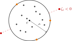
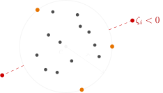
One-class SVM (schematic): a ball with centre and radius encloses the main part of the sample. Objects inside the ball () are not penalised; objects on the boundary of the ball (orange) are the support objects; objects outside the ball (red, ) are outliers, and their penalty grows with the distance from the ball.
One-class classification is a problem in which training objects exist for only one, "normal", class, while objects of the other class, the anomalies, cannot be collected or are too few. Then the region where the normal objects lie is described: here it is a ball of minimal radius. The coefficient sets the trade-off: the larger it is, the smaller the ball and the more objects end up outside. The penalties work as in SVM, piecewise linearly, so the properties of the solution are the same too, including the possibility of replacing the inner product by a kernel to obtain a region of complex shape.
Learning from a sample of one class
Definition (A special case of SSL: PU-learning (Positive and Unlabeled)). Examples of problems where objects of only one class are known:
- detecting fraudulent transactions;
- recommender systems, ad personalisation;
- automatically extending a knowledge base with facts.
A two-class classification model . Unlabeled objects are treated as negative with weight :
One of the successful methods is Biased SVM.
Gang Li. A Survey on Positive and Unlabelled Learning. 2013. J. Bekker, J. Davis. Learning From Positive and Unlabeled Data: A Survey. 2020.
In PU-learning only the positive objects are labeled, and the rest, , are not: among them there are both positive and negative ones. In a recommender system, for example, we know what the user bought, but not what they disliked: an item not bought might simply have gone unnoticed. The simplest approach is to treat all unlabeled objects as negative, but with a small weight, so that errors on them are penalised less than on the reliably labeled positive ones. This is a special case of semi-supervised learning: the same principle of a sum of two criteria with a common model.
Problems with new or unknown classes
Definition (Classification problems with a non-fixed set of classes).
- Ordinary multiclass classification.
- Further training of the model on each new class.
- Detecting the objects of one class (one-class classification).
- Detecting objects of new classes in the test sample (open-set recognition).
- Automatically extending the set of classes with further training of the model (open-world recognition).
Walter J. Scheirer, https://www.wjscheirer.com/projects/openset-recognition
In ordinary classification the set of classes is fixed, and every object belongs to one of them. In practice classes appear over time: new people in a face recognition system, new topics in a document classification system. The problems line up by degree of "openness": from closed multiclass classification to open-set recognition, where the classifier must be able to say "this is none of the known classes", and further to the open world, where the new class must also be added to the model and the model retrained.
Summary
Remark (Summary).
- The nature of anomalous objects: noise (errors, interference, dirt) in the source data; the model describes admixtures of extraneous phenomena poorly; something fundamentally new appears regularly.
- A simple way to weed out the grossest outliers is to exclude the objects with the largest losses.
- A rare case for machine learning: what is minimised is not the sum of losses but a generalised mean .
- The nature of anomalous classes: training objects of a class cannot be collected; the number of classes grows dynamically.
- There is no ideal way to define anomalies. A "model of the anomaly" is assumed, explicitly or implicitly.
No comments yet
Be the first to share your thoughts.