August 30, 2026 · Lecture · LibreTimes
Machine Learning 1. Lecture 11. Advanced Ensemble Methods
Contents
- What this lecture is about
- Reminder: ensembles of models
- One more justification of ensembles: bias and variance
- The problem setting
- The decomposition of the error into noise, bias and variance
- Model complexity
- The bias and variance of simple voting
- Why complex ensembles do not overfit
- Gradient boosting
- The problem setting
- A parametric approximation of the gradient step
- The gradient boosting algorithm
- Example: two spirals
- Stochastic gradient boosting
- Special cases: regression, AdaBoost, AnyBoost
- Variants of loss functions
- XGBoost
- The analytical solution for the leaf values
- The advantages of XGBoost and other variants
- CatBoost
- The main motivations
- Ordered boosting
- The modification of gradient boosting
- Categorical features
- What was left outside the lecture
- Seminar
What this lecture is about
Today is the second lecture on ensembles. I called it "Advanced ensemble methods"; it could have been called more modestly, "Ensembles, number 2". But, as I promised last time, today we will really get to know gradient boosting and the important method CatBoost, which is used very often. It is open-source software from Yandex: for many years Yandex used boosting over decision trees in practically all its machine learning technologies, and then they decided to make an advanced version open. A really great thing; I will tell you a little about how its main algorithm works.
Reminder: ensembles of models
I will begin by recalling what was at the beginning of the last lecture, the general definition of an ensemble.
Definition (The problem of training an ensemble of models). Given: , the training sample;
- , "weak" trainable base models;
- , algorithmic operators with parameters ;
- , a decision rule of a simple form (without parameters);
- , a convenient space of estimates.
Find: an ensemble , where is a correcting function with parameters .
The criterion for training a "strong" algorithm as an ensemble of base algorithms that are "weak" taken separately:
We have a training sample — it does not much matter whether it is regression or classification — there are "object–answer" pairs, there are trainable base algorithms, and we want to build one strong algorithm, a composition, out of a large number of weak ones. For this we single out the main part in the construction of a base algorithm, the algorithmic operator, or, as is often said in classification problems, a real-valued classifier. It works in a space that is in some sense more convenient than the final set ; for example, these are estimates of the degree of membership in the classes. They contain richer information, not yet coarsened by the decision rule, and so it is of course more interesting to build the correcting operation in the space of this richer information. An ensemble, accordingly, is the superposition of the decision rule, the correcting operation and the base algorithms . This is our basic terminology, in which we discussed all this in the last lecture and will continue today.
Definition (Correcting (aggregating) functions). General requirements on the aggregating function :
- , a Cauchy mean, ;
- is monotonically non-decreasing in all .
Examples: simple voting ; weighted voting , , ; a mixture of experts with competence functions : .
General requirements on the aggregating function: it is a generalised Cauchy mean, that is, the result of the correction lies in the range from the minimum answer of a base algorithm to the maximum one; we have no right to go outside this range. Any functions of that fall into this range are exactly the generalised Cauchy means: the arithmetic mean or some other mean, there is a mass of variants. The second requirement is that be monotonically non-decreasing as a function of arguments. For generality I also add the argument : we will consider mixtures of algorithms, mixtures of experts, where really is used inside the correcting operation. And in everything we went through last time — simple voting, weighted voting — the correcting operation did not depend on ; it really corrects only the answers of the base algorithms: for example, averages them, possibly with weights .
One more justification of ensembles: bias and variance
Now let us discuss one more interesting question: one more justification of why this works. Last time I gave the justification of Schapire and Bartlett; we discussed it only at the level of the statement, without proof, because it really is hard. Now I will give an alternative justification of why compositions work, and for this I will need the so-called bias–variance decomposition. I could have told this topic in other places of the course, but it had to be told somewhere, so it went here. Perhaps it would deserve a separate lecture, although it seems to me that it is still very much an auxiliary tool for understanding how individual regression or classification algorithms work.
It was first devised for regression, and I will now show this classical, textbook variant. Conceptually it carries over to classification, but this transfer is not very trivial: technical difficulties arise that I would rather not discuss within the course. So I will show the rigorous results for regression problems, and still illustrate them as applied to classification. There is a certain stretch in this, but not too great.
The problem setting
Definition (Bias–variance analysis).
- A regression problem: .
- The quadratic loss function: .
- The probabilistic setting: .
- The learning method: , i.e. sample algorithm.
The problem of minimising the mean squared risk:
The ideal minimiser of the mean squared risk:
The main quality measure of the learning method :
Suppose we have a regression problem and the quadratic loss function, so as to use the least squares method. The probabilistic setting tells us that the "object–answer" pairs of the training sample and of the subsequent test sample come from one and the same distribution on pairs. There is a learning method: it takes a training sample as input and outputs an element of a parametric family of functions . That is, an algorithm is built from the sample, it is trained, some optimisation problem is solved.
We are interested in what losses the trained algorithm gives on an arbitrary pair generated by the unknown distribution . Let us write the formula: it is the expectation of a random variable, the squared deviation, an integral over the distribution both in and in . In principle, in training we ought to minimise it over . But since the density is unknown, we cannot pose such an optimisation problem explicitly, so we optimise what we have — in effect the sample estimate of this integral, the mean loss over all the objects of the training sample. Having substituted the optimisation problem in this way, we naturally come to bias and overfitting. Overfitting is precisely the bias of the estimate we get on the training sample itself: it will be optimistic, we will underestimate the mean squared risk.
Let us agree that the ideal minimiser of the mean squared risk for us will be the function , the conditional expectation of at the given point . It is by no means obliged to lie in : after all, is our model, usually a parametric family of functions from which we choose an approximation. The conditional distribution is taken from the same density that describes reality, and we do not know it. But purely mathematically, formally, we can introduce this definition: is the ideal minimiser of the mean squared risk; it is the very dependency we are trying to recover. It is hard to recover both because the density is unknown to us and because the family of functions that we use as a model may not contain .
Now let us characterise generalisation ability. The main quality measure of a learning method is the expectation of the function . itself is the expectation over one test object for a particular approximation ; it estimates the risk of a particular function. And now as the particular function we take the one obtained at the output of the learning method from the training sample , and we take the expectation over all training samples as well. Here there is in effect a double expectation: over the training sample and over one test example. We built an algorithm from the training sample, applied it to one test object, and estimate the expectation of the squared difference. This is the characteristic of generalisation ability that ideally we should minimise — the characteristic of how well we are able to learn, computed on an independent examination object. The trouble is that we cannot compute it, since the density from which both the training sample and the examination example come is unknown. But something, theoretically, under uncertainty, we can understand — at least structurally, what consists of. This is the decomposition of the error into three components.
The decomposition of the error into noise, bias and variance
Definition (Notation).
- is the unknown ideal dependency of on ;
- is the observed answer on the object ;
- is the algorithm from the model trained on the sample ;
- is the mean answer of the trained algorithm.
Once more: is the expectation of at each point , the unknown ideal dependency, in effect the target dependency we are trying to approximate but do not know. is the observed answer on the object , taken from a conditional distribution that we also do not know. is the result of training by the method on the training sample : an approximation chosen from the model family , which in principle should approximate .
And one more notion, the mean answer of the trained algorithm : the expectation of the result of training over all possible training samples. Expectation in the sense of an integral over all training samples, over a density that is unknown to us, and over the whole space of training samples too. Clearly this is a non-constructive thing, we cannot compute it, but we can introduce it purely mathematically. Such an expectation at a particular object is a function of , and it is an interesting thing for us, because it is an integral approximation of simple voting. It is as if we had voted over absolutely all the algorithms that can be built from all possible training samples. There are infinitely many of them, so we cannot simply sum and average them, but the integral is, in the limit, exactly the averaging over an infinite ensemble of algorithms trained on one and the same problem from different samples. By the problem we mean the distribution , which is of course unknown to us.
Theorem. With the quadratic loss function, for any
I will not prove the theorem — not because it is hard, but because its proof is in many textbooks, it is simple, and you can even reproduce it yourselves in about ten minutes.
Proof. It is done very simply: into the difference we add and subtract two functions, and . The square decomposes into a sum; we open the brackets, transform a few things, and in the end we get a sum of three components, each of which has the meaning of the expectation of some squared deviation.
Now let us look carefully at what these squared deviations are and try to interpret them. So, is the expected error on an examination example after training on a random training sample, and it has three components.
The first is called noise. is the function we want to approximate. But noise may be superimposed on : is the expectation of given , and the we have in the training sample may deviate from this function because of random noise. In we have removed this noise, taken its expectation. That is, noise is the deviation of the ideal dependency we dream of recovering from the real we see as the results of observations. Measurement noise may be superimposed on these results, the noise of the instrument with which we measure , and this noise is irremovable. Clearly in machine learning we cannot and must not approximate these noises or build a model of them at all; we do not do that. Noise is an irremovable element of this decomposition.
The second component is the distance, on the examination example , between the mean answer of the trained algorithm and the ideal unknown dependency . The mean answer of the trained algorithm can be considered as lying inside the family : although it is the result of an expectation, it is still an element of the parametric family. How far it deviates from is called the bias, the bias of the model relative to the true dependency . All these objects — , — are functions of , elements of a function space. And most likely lies outside the family . Why? Because the space of functions is, generally speaking, infinite-dimensional, while the parametric model is finite-dimensional: it is simply a set of measure zero in the function space. The function , which can be anything at all, is unlikely to fall into our parametric family: it is too "flattened" for a random element of the function space to land right in a finite-dimensional subspace. So the bias shows how unluckily we chose the model, how far we have managed to devise a parametric model that comes close to .
The third component contains the expectation both over the training sample and over a separate examination example. We do not land on the mean result of training , but choose some particular element of the parametric family , and this particular element carries the result of training on a particular sample. This is the variance, the variability of the result of training, connected with the randomness and finiteness of the training sample. Clearly, if the training sample is small, if there are not enough data, the variance will be large: the less data, the larger the variance and the larger its contribution to the total error.
Remark (Two different averagings). Here it is easy to get confused about which average is meant. When we gave the general definition of bias and variance, we talked about the mean answer of the trained algorithm , and this average is non-constructive, non-computable: it is an expectation, an integral over all possible training samples. If we average base algorithms, that is at least some approximation to this integral, to . But that was the general theory, full stop. Next we are interested in how it applies to ensembles, to simple voting. Now we say that our model is arranged like this: it is the result of averaging base algorithms taken from some parametric family and trained somehow on the sample. Only at this moment did we say that is simple voting. We substitute such an ensemble into the formulas for bias and variance and see what comes out; I omit the substitution itself, it is a purely technical thing you can manage yourselves.
Model complexity
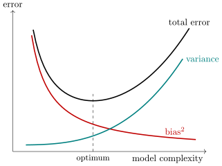
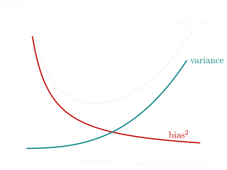
As the complexity of the model grows, the bias decreases and the variance increases; the total error (with the irremovable noise) is minimal at some optimal complexity. Schematic.
Let us discuss in substance what bias and variance are — a qualitative understanding of how they depend on the complexity of the model. When you increase the number of parameters in the parametric model , you will of course reduce the bias: you make the model richer, it will be able to get closer to the point . So the bias decreases as complexity grows. But the variance may increase. Why? Because as the number of parameters grows, overfitting will begin: you will spend the excess degrees of freedom of the parametric family on adjusting to the noise or to the peculiarities of the particular data sample. So the bias will decrease and the variance increase, and I show this schematically on the plot.
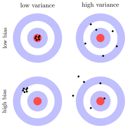
Bias and variance on a target: bias is a misaligned sight (the shots are grouped but not in the centre), variance is an inexperienced shooter (the shots scatter over the target).
Also pictures with a target — just to remember how bias differs from variance. Bias is when your sight is out of alignment. And variance is when you are an inexperienced shooter and keep missing the target.
The bias and variance of simple voting
Why all this, and how does it relate to compositions? Let us look at the situation where we have base algorithms trained on random subsamples — practically the bagging we considered last time — and the ensemble is simple voting. One can substitute it into the formulas and get more precise expressions for the bias and the variance. Again I do not prove this; it is a technically quite simple exercise; let us just look at the result and interpret it.
Proposition. Let the base algorithms be trained on random subsamples: , , , and let the ensemble be simple voting:
Then the bias of the ensemble coincides with the bias of a single base algorithm:
and the variance consists of the dispersion and the diversity (covariance), :
The bias of the ensemble coincides with the bias of a single base algorithm, and this is very good news. It says that because of averaging, simple voting, the error — at least its bias component — cannot increase: whatever bias the individual base algorithms had, the composition will have the same. By averaging base algorithms from a model, you can neither improve nor worsen its accuracy in the sense of bias.
The variance is more interesting: it too, it turns out, consists of two components. The first is the dispersion of the individual base algorithms, and it is divided by . And the second is the covariance, and it shows that if the base algorithms are different, the second term will decrease. This is exactly what we originally built into compositions and discussed at the very beginning of the last lecture: it is useless to average base algorithms that are too similar to each other. An improvement will arise only if they approach the condition of averaging independent observations of a physical quantity. Ideally they should tend to independence, but they will never be independent, simply because they are trained to solve one and the same problem; they are certainly dependent. So here we speak not of independence but of diversity — a more correct term that does not presuppose statistical independence. And the more diverse the base algorithms, the better.
This explains what bagging does: it averages different algorithms and tries to make them different by training them on different random subsamples. Boosting in essence does the same: it increases diversity by training the base algorithms on differently weighted samples, where each next time large weights go to the objects that turned out to be the hardest for all the previous base algorithms. That is, the mechanisms for increasing diversity in bagging and boosting are different. That is good: both methods are voting, but they do it differently.
Why complex ensembles do not overfit
From the standpoint of margin analysis:
- ensembling does not increase the complexity of the model,
- but with each iteration it increases the gap between the classes.
From the standpoint of bias–variance analysis:
- the diversity of the base algorithms reduces the variance;
- bagging reduces only the variance;
- boosting reduces both the bias and the variance.
A practical comparison: boosting / bagging / RSM:
- boosting is better for classes with boundaries of complex shape;
- bagging and RSM are better for short training samples;
- RSM, when there are many dependent and uninformative features;
- bagging trains the base algorithms in parallel;
- boosting trains each in parallel over parts of the sample.
What matters to us now is a conceptual understanding of why complex ensembles do not overfit. Last time I told one justification — from the standpoint of margin analysis: ensembling does not increase the complexity of the model, but with each iteration it increases the gap between the classes; this is how boosting acts. Now from the standpoint of bias–variance analysis. This is a completely different theory, and its conclusions are a little different: the diversity of the base algorithms reduces the variance, and that is good. Both boosting and bagging reduce it, each in its own way. Bagging reduces only the variance and in no way tries to reduce the bias. But boosting reduces the bias too: this was studied at the end of the nineties, when people tried to give theoretical justifications of why boosting works. Boosting reduces the bias by training the base algorithms on specially weighted samples, and builds a much more complex separating surface than a single base algorithm could afford. Bagging, on the other hand, only averages, that is, only reduces the variance.
The practice of comparing boosting, bagging and the random subspace method (RSM) allows the following conclusions; there were many publications on this subject, and without going into these studies I give only the ready conclusions. First: boosting suits classes with boundaries of complex shape better. Bagging is too simple — it is simple voting over algorithms trained on subsamples — while boosting is subtler: it reweights both the objects and the base algorithms in weighted voting, and so solves more complex problems. The random subspace method is better when we have many uninformative features: by building random subsets of features, we may come across ones that work well, and this will be reflected in the quality of the base algorithms — on the one hand they will be diverse, and on the other, not bad individually.
Further: bagging trains the base algorithms in parallel. Boosting can be parallelised too, but since the base algorithms are built strictly sequentially, one after another, it is the construction of each base algorithm that has to be parallelised. These technologies have been mastered; this is exactly what Yandex worked on when it made its MatrixNet, and then CatBoost, and there are many publications on this subject, and not only from Yandex. But parallelising the construction of a base algorithm is much harder than simply handing out the tasks of building base algorithms independently on different training subsamples.
These are the conclusions from comparing boosting and bagging from the point of view of different theories of overfitting — margin analysis and bias–variance analysis. That is the end of this story; it was a small theoretical insert and an occasion to tell about the bias–variance decomposition, with which of course one can justify not only compositions. Bias and variance estimates are known for regression, for metric methods, for nearest neighbours and many others; such theories have been built, but discussing them is not the subject of our course. They give interesting estimates, but these estimates cannot always be turned into real constructions of classifiers; very often they are catastrophically loose and give only a general understanding of how learning methods could be built, and do not always give constructive conclusions. This is the reason why I do not present the theory of generalisation ability and the various approaches to it in a general machine learning course: here we talk more about methods, and our task is to study practical algorithms, not theoretical estimates, which, unfortunately, are often impractical.
Gradient boosting
And here is a very practical piece I would like to tell — gradient boosting. It did not appear at once, but four years after Freund and Schapire devised AdaBoost, and it appeared as a generalisation. After AdaBoost people began writing a pile of papers: let us take, instead of the exponential loss function, some other one, for example as in logistic regression — and many other variants. And then Jerome Friedman wrote a paper that generalised all this: these separate studies need not have been done; one could simply substitute into Friedman's general formulas the various loss functions that can be devised in classification problems.
The problem setting
Definition (Gradient boosting for an arbitrary loss function). Given: , .
Find a linear ensemble of base algorithms :
Heuristic: we train , with the previous ones fixed.
The criterion with a given smooth loss function :
is the vector of the current approximation.
J. H. Friedman. Greedy function approximation: a gradient boosting machine, 1999.
Let us consider a linear ensemble of base algorithms. The base algorithms are taken from some parametric family , in particular they may be decision trees, and we are doing weighted voting — determining the coefficients for the base algorithms. The heuristic is very similar to AdaBoost, only, unlike AdaBoost, here the loss function is considered in general form. The main thing is that it be a smooth function of the algorithm's answer, of the first argument; otherwise it can be anything — and not only for classification, for regression too. It does not matter how we compare the correct answer with the model's answer, the main thing is that this function be smooth. The heuristic that we train the next stays the same as in AdaBoost: the whole part relating to the previous base algorithms is considered fixed.
Let us introduce notation. The fixed part, the composition of base algorithms with all its , we already know by the moment base algorithm number is built. So on each training object we can compute the answer of this composition, , and collect all these answers into a vector. We will say that this is the current approximation: the current composition of base algorithms returned these answers on all the objects of the training sample. The vector is made up of base algorithms: we will add the next base algorithm and determine its coefficient. Our task is to pass from the vector of the current approximation, which we already know, to the vector of the next approximation, by specially building a base algorithm for it and determining the coefficient , that is, to solve an optimisation problem over the base algorithm and its coefficient in weighted voting.
A parametric approximation of the gradient step
Why did we introduce these two vectors, of the current and the next approximation? In building a base algorithm, we move in the space of answer vectors of dimension — the size of the training sample — from one point to another. Having built a base algorithm, we must find a new point in the answer space that is better in terms of the sum of losses. That is, in effect we solve the problem of minimising the functional over and so as to pass, in the space of vectors of dimension , from the current approximation to the next one. The functional is the sum over all objects of the loss function of the composition's answers on all the objects of the training sample, of these vectors.
Definition (A parametric approximation of the gradient step). The gradient method of minimising , :
- the initial approximation;
- , ;
are the components of the gradient vector, is the gradient step.
This is very similar to adding one base algorithm:
The idea: look for a base algorithm such that the vector approximates the antigradient vector :
Suppose for a second that we could freely choose the vector in this space. Of course this is not so: we can pass to the vector of the next approximation only by building the next base algorithm, and this constrains which vector we can get at all. But let us suppose that there are no constraints and we can get any vector . How would we act then? We would act by gradient descent, we would take a gradient step: from the vector we would pass to the vector by subtracting the gradient vector with gradient step . The vector consists of the derivatives of the loss functions with respect to all the components of the vector , and is the gradient step.
And now let us consider adding one base algorithm to the composition, and to our surprise find a formula of almost the same form. is the composition of the previous base algorithms, and is what we add to this composition, and it is very similar to minus the gradient. Hence the idea: why not build the base algorithm so that it simply approximates the antigradient vector? Then is simply the gradient step. We will choose base algorithms from the family so as to approximate, by least squares, the antigradient — the derivative of the loss function with respect to the first argument, computed for the previous composition at each object of the training sample, for all from one to .
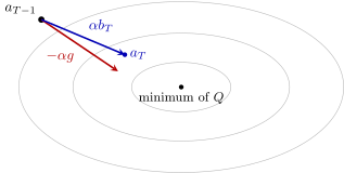
Gradient boosting in the space of answer vectors on the training sample, (schematic): from the current approximation , the gradient method would step along the antigradient , while boosting steps along the vector , the answers of the base algorithm closest to the antigradient in the least squares sense. The ellipses are level lines of .
So look: regardless of the loss function, regardless of which problem we are solving — it may be regression or classification, and the loss function may be anything — we will build the base algorithms by least squares, as if we were solving a regression problem. Even if in fact we are solving a classification problem. It is just that in this regression problem we approximate not but the antigradient vector at the point of the previous composition. This is the essence of the gradient boosting method. Now it is clear why it is called gradient: we have found an analogy between building the next base algorithm and a gradient step in optimising the vector of the composition's answers on all the objects of the training sample.
An interesting analogy between unconstrained gradient optimisation — here the vector is arbitrary — and building the next base algorithm in weighted voting. And it is interesting that the size of the gradient step coincided with the weight coefficient of the base algorithm; this too is rather unexpected. This is a non-trivial generalisation of weighted voting to an arbitrary loss function, and it goes through the analogy of building one more base algorithm with one more step of gradient optimisation of the same criterion. The non-trivial conclusion is that boosting is in fact approximate gradient optimisation: building the next base algorithm is as if taking one more step of gradient descent in a space of dimension . In my view this really is a subtle, non-trivial and beautiful point; finding such an analogy was a non-trivial achievement.
The gradient boosting algorithm
Definition (The gradient boosting algorithm (Gradient Boosting)). Input: the training sample ; the parameter .
Output: the base algorithms and their weights , .
- initialisation: , ;
- for all :
- a base algorithm that approximates the antigradient:
- a one-dimensional minimisation problem:
- update the vector of values on the sample objects: , .
Each next base algorithm is trained so as to correct, as far as possible, the errors of the previous algorithms.
Let us write the method as pseudocode. In architecture it is very similar to AdaBoost. What they have in common is that all the base algorithms are built in turn, one after another, and that the number of base algorithms is set in advance: we agree in advance how many we will build. Inside there are two main steps. The first: we build a base algorithm, but in this case always by least squares, fitting it to the antigradient. The loss function is smooth, we always set it and know it in advance, and we can always compute its derivative, so this causes no problems.
The second step is a one-dimensional minimisation to determine . This is already a substantial difference from AdaBoost. In AdaBoost the loss function was fixed — the exponential — and we expressed analytically, wrote out a formula into which simply has to be substituted. Here it is harder: of course appears, but in the problem has to be solved by an optimisation method, because the function can in general be anything. Bisection, Newton's method, anything at all will do — it is not hard, but there is, alas, no analytical formula. Everything has its price: for generality one often pays by getting a numerical method instead of a short, simple analytical formula.
And the last step: we prepare for the next iteration, updating the vector of values on all the objects of the sample. The general principle of boosting — both in AdaBoost and in its generalisation, gradient boosting — stays the same: each next base algorithm is trained so as to correct, as far as possible, the errors of the whole previous composition. This is a common feature of all boostings, and gradient boosting, since it is the hyper-mega-super-generalisation of all other boostings, keeps to this principle too.
Example: two spirals
Let us look at an example; many such examples can be found on the internet. I chose a nice problem on synthetic data (the slides show pictures from A. Rogozhnikov's interactive gradient boosting "playground"): a two-class classifier has to separate two nested spirals. Boosting over 100 trees of depth 5 is built, and the first 30 trees are shown. It looks like a spiral in places, and in places not very: decision trees have an angular logic and approximate such boundaries poorly. At the bottom the losses in training and on test are shown, and one can see that the overfitting is quite considerable: the training loss is 0.022 and the test loss 0.218, ten times larger. Nevertheless the test error does decrease as the number of base algorithms grows; this function is decreasing. There is overfitting, but not catastrophic, and it is due rather to the bias of the base family: trees are poor approximators for such spirals. The number of base algorithms increases here, but this does not lead to overfitting: they are simply averaged.
And the next picture illustrates how trees are rotated. A tree is built in full, and then an angle of inclination is chosen for it. This is not rotating the features in each internal vertex of the tree — such methods exist too, but they are called oblique decision trees, a different construction. Here the tree is rotated as a whole after it has been built. This base family turns out to have a smaller bias on this particular problem: rotated trees are a little better at describing spirals. This shows in the overfitting being much smaller: losses of 0.013 in training and 0.092 on test. The model over rotated trees turned out more than twice as good as over unrotated ones. This is a small illustration of the fact that the choice of the family of base algorithms matters, although many theoretical results say that base algorithms should be as simple as possible; in practice this is not always so.
Remark (The light zones in the picture). There are two classes in the picture, the blue and the yellow objects, and the light shades show the level of confidence: the trees here are probabilistic, and light yellow and light blue show the zones of uncertain classification. As far as I understood this example.
Stochastic gradient boosting
One more interesting generalisation was devised by the same Jerome Friedman in a paper of the same year, 1999: stochastic gradient boosting. He asked himself: in gradient boosting, the most general boosting, we still build each base algorithm on the whole training sample. True, each time we fit the base algorithm a little differently, to a different antigradient vector. But can the same idea as in bagging be used? Friedman tried, and it turned out that this really does improve the quality of the composition.
Definition (Stochastic gradient boosting (SGB)). The idea: when optimising and , use not the whole sample but a random subsample, by analogy with bagging.
Advantages:
- convergence improves and training time decreases;
- the generalisation ability of the ensemble improves;
- unbiased out-of-bag estimates can be used.
The conclusion of experiments: it is optimal to sample about 60–80% of the sample.
J. H. Friedman. Stochastic gradient boosting, 1999.
This is indirect evidence that gradient boosting had not yet squeezed out everything that could be squeezed out. The variance can decrease when the diversity of the base algorithms increases, and gradient boosting did not do everything it could to reduce the variance. In practice it is almost always stochastic gradient boosting that is used: when optimising and in the pseudocode I showed, we are not obliged to sum over the whole sample but can take random subsamples, roughly as is done in bagging, not necessarily with replacement.
What does this give? Training time is reduced: if we train on a sample half the size, we will do this work twice as fast. The generalisation ability of the ensemble improves. And also, since each base algorithm is now trained not on all the data but only on part of it, it becomes possible to use unbiased out-of-bag estimates exactly as was done in bagging over decision trees, in Random Forest.
The experiments (the slide shows plots from Friedman's paper) show the relative error for various sizes of the random subsamples on which the base algorithms are trained. It turns out that if the share of objects in training is 100%, that is, if we train on the whole sample, as in the basic variant of gradient boosting, the result is worse than when we take 70%, 80%, even 90%. This depends on the problem: one can see that on one problem the best result is obtained at a share of 0.6, and on another at 0.8. But this is a fairly general recommendation: many problems were tried, and a sample of 60 to 80% works best.
Special cases: regression, AdaBoost, AnyBoost
Why is gradient boosting a generalisation of all other boostings? Let us look at a few special cases.
Example (Special cases of gradient boosting). Regression: :
- is trained on the differences ;
- if the regressions are linear, need not be trained.
Classification: , : gradient boosting coincides exactly with AdaBoost [Freund, Schapire, 1995].
Classification: , : gradient boosting coincides with AnyBoost [Mason et al., 2000].
L. Mason et al. Boosting algorithms as gradient descent, 2000.
Let us start with regression. The loss function is the squared difference, and then gradient boosting means that we simply train the next base algorithm on the differences, on the residuals: the derivative of the squared difference is exactly the residual up to a factor. This method was invented and reinvented many times by many authors long ago, even before the word "boosting" arose. No particular attention was paid to it: it was used in practice — fine. There was no awareness that it was a special case of something as wonderful as gradient boosting.
Next, one can take the exponential loss function and write out what happens with gradient boosting, purely theoretically: take and solve analytically the problem of determining the coefficient . This goes through, and we get exactly AdaBoost.
There is one more generalisation, not as general as gradient boosting — for classification with a loss function of the form "a decreasing function of the margin". It was called AnyBoost: it is for any classification problems with any loss functions, but only for classification. Other problems, for example regression with the quadratic loss function, no longer fall under this case, because the generalisation here consists in taking an arbitrary smooth decreasing function of the margin and carrying the learning method through to pseudocode. I do not tell about this in the lectures, because it is simply a special case of gradient boosting, although the derivation there is done a little differently, not through the analogy with gradient descent. The paper even came out a year later than Jerome Friedman's paper.
Variants of loss functions
I have shown several times the picture with the approximations of the threshold loss function (it is in the previous lecture).
| Loss function of the margin | Boosting variant | |
|---|---|---|
| exponential | AdaBoost | |
| logarithmic | LogitBoost | |
| quadratic | GentleBoost | |
| Gaussian | BrownBoost | |
| sigmoid | ||
| piecewise linear | from SVM |
The threshold loss function (red) and its smooth approximations as functions of the margin (slide); the notation is as in the table.
AdaBoost is the exponential approximation of the threshold loss function, and there are also numerous LogitBoost, GentleBoost, BrownBoost — whatever was not devised, about twenty such names. But then gradient boosting appeared, and it became clear that these different variants can be changed like gloves. Each loss function may have some interesting properties. In particular, BrownBoost's loss function has a decreasing branch that makes it possible to ignore large outliers — rare objects that have ended up in another class: let us not train on them. Such a heuristic is easy to build into gradient boosting through the loss function. With this the story of general gradient boosting ends.
XGBoost
Now one more variant: XGBoost — please welcome it, and use it often when solving applied problems. A good thing, and people really do use it very often in all kinds of data analysis competitions. It is a special kind of gradient boosting in which regression and classification trees, CART, are used as the base algorithms.
Definition (XGBoost: a popular and fast implementation of gradient boosting over trees). Classification and regression trees (CART):
where is the binary indicator falls into the leaf , is the value in the leaf , is the set of leaves of the tree. For any one and only one term is non-zero.
The quality criterion with the sum of and regularisers:
where is the previously built part of the ensemble.
Tianqi Chen, Carlos Guestrin. XGBoost: A scalable tree boosting system, 2016.
We have already talked about this: a tree is a variant of a linear classifier. Let us introduce the binary indicator that the object falls into the -th leaf of the decision tree. Each object falls into one and only one leaf — this is so by construction for any decision tree. If in the -th leaf vertex you return the value at the output, the tree can be written as a linear classifier. This is a purely formal notation: among the terms — is the number of leaves of the tree — for each point one and only one is different from zero, and all the others are zero, because the object falls into exactly one leaf: equals one only for this leaf. Formally it seems to be a sum, but there is always only one non-zero term in it. This is a convenient notation that lets one realise that a decision tree is in fact a linear classifier over binary features. And it is clear by what formula each feature is written: it is the condition that the object has fallen into the given leaf, that is, the conjunction of all the conditions in the internal vertices that led it from the root of the tree to this leaf.
Since it is a linear classifier, let us train the indicators as if they were base algorithms and we were building boosting over them. We need a criterion. Take the sum over all objects of the training sample of the loss function; we have the previously built part of the ensemble — exactly as in gradient boosting — and we add a whole tree to it, that is, a whole lot of terms at once, and we will determine the weights of all these terms simultaneously. Since it is a linear classifier, it can overfit, and to keep it from overfitting, let us add regularisation: we will penalise the squared norm of the vector , the sum of the squares of the coefficients sitting in the leaves of the tree. And let us also introduce regularisation: a penalty on the number of leaves . The regularisation coefficients and have to be chosen somehow.
The analytical solution for the leaf values
Why did we cook up this whole complicated mess? So that, despite the generality of the loss function, we could get as far as possible with an analytical solution of this optimisation problem.
Definition (XGBoost: an approximate analytical solution for). We approximate
where , , .
From the conditions we find the optimal value of the leaf :
Substituting back into , we derive the splitting criterion:
For this we will of course resort to a trick. The trick is that we add a correction to the ensemble and consider it not very large. And since the correction is small, let us use the Taylor expansion to second order: the loss function , its first and second derivatives, in the small correction . If is treated as a correction, the point is the whole previous composition, which we know, and in a neighbourhood of the point we make a second-order approximation of our loss function. Substituting it into the functional, we get the problem of minimising the approximated functional with respect to , and is a linear combination of binary indicators with coefficients (the term does not depend on and drops out).
Now it is clear why we took exactly the second order and why we needed the second derivatives: the term with is expressed through the squares of , and we also have the squares of in the regulariser. The first order would not do here. This simplifies the problem greatly. Let us recall once more that in the sum one and only one term is non-zero: the are the indicators that the -th object falls into the -th leaf, and on any object it is one for only one out of all, and the rest are zeros. is the answer of our whole tree on the -th object, and we need it to the first and second power. The power is computed very easily: it would seem that the whole sum has to be raised to the power, but only one term in it is non-zero, so the -th power of the sum is the sum of the coefficients to the -th power multiplied by the indicators. We have greatly simplified the form of the formula. and are simply new notation for the first and second derivatives.
This problem can now be solved analytically: differentiate with respect to and set the derivative to zero. This is why XGBoost is so efficient and fast: no optimisation problem has to be solved to train a base algorithm; the required coefficients sitting in the leaves of the trees are computed by analytical formulas. I skipped half a line of calculations, but it turned out easy. The value in a leaf is computed by this formula as soon as we understand which objects exactly have fallen into this leaf: are the indicators that the training object falls into the -th leaf, and as soon as we have understood which objects of the training sample have fallen into the leaf vertex, we can compute from this subsample what value should be in the leaf. It is an interesting sample estimate — two sums, of and of , the values of the first and second derivatives of the loss function, divided by each other.
And now it becomes possible to write out the splitting criterion for building the trees as well. What do we build them with? With ID3, of course, what else; in CART, classification and regression trees, the splitting principle for building internal vertices is the same as in ID3. After substitution we get a formula by which the decision is made which feature to use in each internal vertex. This formula requires nothing of us except computing sums over the training objects that have reached the given vertex — it is in essence a splitting criterion like all the others: we computed sums, divided them by each other, and by this criterion we choose a feature in each vertex. Thanks to the analytical formulas for the coefficients in the leaves and for the splitting criterion, the tree trains fast. These formulas optimise the functional , which in turn is the second-order approximation of the original functional , written exactly as in gradient boosting: the next base algorithm is optimised with the composition of the previous ones, , already known. Such is the XGBoost method; it shows that the problem of optimising a base algorithm can be dealt with analytically even if the base algorithm is not very simple — a classification or regression tree.
The advantages of XGBoost and other variants
The advantages of XGBoost (eXtreme Gradient Boosting):
- regularisation reduces overfitting;
- regularisation simplifies the trees (pruning);
- like general gradient boosting, it allows arbitrary loss functions;
- a very fast implementation thanks to the analytical formulas;
- it has a mechanism for handling missing values.
What else there is:
- LightGBM, for training on very large data;
- Yandex.MatrixNet, gradient boosting over oblivious decision trees;
- Yandex.CatBoost, for categorical features.
G. Ke, Q. Meng, T. Finley, T. Wang, W. Chen, W. Ma, Q. Ye, T.-Y. Liu. LightGBM: A highly efficient gradient boosting decision tree, 2017.
A couple more words about XGBoost — from the words eXtreme Gradient Boosting. It is good in that it even has two regularisations. regularisation makes it possible to reduce overfitting, because it is a linear classifier. This is also the answer to the question of why we went to the trouble of forcing the decision tree into the form of a linear classifier: so that the same regularisation that we apply to linear classifiers could be applied to it. More than that, so as to realise that in building a composition we are in effect building a linear composition of such linear classifiers. Imagine: if we build 100 decision trees and each has 100 leaf vertices, then in effect we have built a linear combination of 10,000 binary indicators. So that this linear composition does not overfit, it makes sense to impose regularisation on it, and the are exactly the values that sit in the leaves of the trees. Such is the interesting connection between a linear classifier and a decision tree, and the justification of why exactly regularisation. And regularisation is simply a kind of pruning.
XGBoost is as general as gradient boosting and allows arbitrary loss functions: of the loss function we need to know only its first and second derivatives, be able to compute them, and otherwise it can be any function. Thanks to the analytical formulas, a fast implementation. And there is also a built-in mechanism for handling missing values, but I do not tell about that; trees can work with missing values.
What other variants of gradient boosting of this sort are there? There is one more efficient implementation, LightGBM; it is quite well suited to training on very large data, but again I will not go into details. There is Yandex's closed and outdated solution MatrixNet — it was not opened; it is gradient boosting over oblivious decision trees. And there is CatBoost, which I will now tell you about.
CatBoost
CatBoost generalised many years of experience of applying MatrixNet in ranking, advertising and many other machine learning problems. Over time it was realised that it is very important to learn to work with categorical features — features that take a finite set of values, but there can be a huge number of these values.
The main motivations
Definition (The main motivations of CatBoost). Two problems:
- categorical features with a large number of rare values have to be handled (user, region, city, advertisement, advertiser, product, document, author, etc.);
- overfitting (bias, target leakage) in the gradients: the are computed at the same points on which the ensemble was trained to approximate .
A trick similar to out-of-bag and to online methods:
- to get unbiased estimates on the object , keep and further train the ensemble on samples without this object;
- how can there be of these samples rather than ?
- how can they be made not to overlap much?
L. Prokhorenkova et al. CatBoost: unbiased boosting with categorical features, 2018.
For example, the feature is the user: you would like to make a complex algorithm that could tune itself to a particular user. Or the city the user lives in — there are also many thousands of cities, and one would like the model to be able to understand that in each city, for example, search should work in its own way: people look for a shop near their home, that is, at least in their own city. How can one learn to take this into account in a very simple way, and without building models explicitly, simply by feeding into the general model a feature, the user ID? Each user is distinguished by their identifier, and if the user ID is used as a feature, one can potentially count on the model taking into account somehow the history of this user: what search queries they made, what their interests are, and so on. A lot could be done if we could simply identify the user. But we do not want to do feature engineering explicitly, to invent features that depend on the user. Let us just throw the user ID, or the ID of the city they live in, at the model.
This was the original motivation — to use such features in models trained on very large data. There may be millions of users, but there are so many data — billions if not trillions of records of user actions — that the hope arises: there were a great many records about each user with such an ID, some transactions, and then the ID really becomes an informative feature. And we have no wish at all to extract further features from the knowledge of a particular user, to construct separate features on such complexly structured objects. We want to throw the ID of the user or the city into the model and forget about it — so that the model itself pulls out all the necessary information. This is the main motivation for why we want to handle categorical features.
And there is one more problem — with this I am moving smoothly to the next story. In boosting, leakage (target leakage), bias and overfitting quite often arise because we compute the gradients from the loss function of the previous composition at the same points on which it was trained. And one would like to get the gradients at points on which the composition was not trained — the same idea as in out-of-bag. Can the out-of-bag idea be carried over into gradient boosting? In general, generally speaking, no, because in gradient boosting each base algorithm is trained on the whole sample. To get an unbiased estimate on an object, it turns out, one has to keep and further train the ensemble on all the samples without this object. This is very hard, and it seems that one would have to keep as many samples as there are objects — that is sheer madness, it certainly cannot be done purely technically. But can one at least reduce the number of these samples so that it becomes logarithmic in the total number of objects? How to do this — the whole trick of CatBoost rests on this very cleverly arranged out-of-bag.
Ordered boosting
Definition (Ordered boosting). The ideas:
- compute from a model that was not trained on ;
- build training subsamples of doubling length;
- build many such randomly shuffled samples.
Notation:
- are random permutations of the sample ;
- is the subsample of the first objects of ;
- is a semi-finished ensemble trained on ;
- is the antigradient at the point for the ensemble , which was not trained on it, .
The idea is called ordered boosting. We will compute the gradient at the -th point from a model — a composition of base algorithms — that was not trained on this object. We will have to build and train such compositions on subsamples of doubling length. And we will build many such random subsamples — many, but not too many: we will keep shuffling the training sample, setting a random order of the objects, say twenty to thirty times.
Where did this idea come from? From incremental learning methods, including methods on time series — we will talk about such later in the course. There the objects arrive in a certain order, and we train a model. And there were such methods: a model trained on some sample is not retrained on each newly arrived object; instead one waits until exactly as many new objects have accumulated as there were before — that is, until the amount of data has exactly doubled. Then the retraining is done, and a new model is built on the training sample that has doubled in size. This idea from online learning on dynamically arriving data was taken as the basis of CatBoost.
Now more precisely. are random permutations of the sample. After all, we are working with a sample given to us at the outset; this is not a dynamic situation, as with time series, when we cannot know the future and are forced to train the model in portions as the data arrive — in fact we have all the data. So, in order still to train the compositions on all the data, let us order the sample: introduce artificially a kind of arrival time for the objects of the training sample, but do it times and differently, that is, sort the sample differently. is the first objects to arrive in the -th permutation; training will go on subsamples whose size will always be a power of two. is an ensemble, but so far a semi-finished one: we have not yet built all the base algorithms. It is trained on the subsample , the first objects in the order of the -th permutation.
We build all these semi-finished ensembles simultaneously, and there are times the logarithm of the data size of them — that is already an acceptable number. We build many ensembles simultaneously so that we always have base algorithms that were not trained on any given object: whatever object we take, we will always find a sufficient number of such ensembles, can make a composition from them and get an unbiased, out-of-bag estimate on this object — for anything, including the gradients. Here they are, these gradients: the antigradients of an ensemble of base algorithms that was not trained at this point.
If we want to take some point, for example the object standing thirteenth in the permutation, which ensemble can we take so that it is guaranteed not to have been trained on this object? By this formula: the floor of the binary logarithm, that is, for the number 13 we take the nearest smaller power of two, 8. is the index of the semi-finished ensemble, the number of the permutation, and the number of the object in the particular permutation. In this way we will find for each object quite a lot of base algorithms that were not trained on it, and among them there will be ones trained on large samples, on not very large ones, and on very small ones.
Ordered boosting (slide): the objects in the order of a random permutation and nested subsamples of the first objects. The gradient on the object in place is computed from the semi-finished ensemble trained on the first objects.
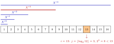
Ordered boosting (schematic): the sample objects in the order of a random permutation and the nested subsamples of the first objects. The gradient on the object standing in place of the permutation is computed from the semi-finished ensemble trained on the first eight objects, that is, without this object.
The modification of gradient boosting
Definition (The modification of gradient boosting in CatBoost).
- generate random permutations ;
- for all :
- choose a permutation at random from ;
- , the unbiased antigradient;
- ;
- for all trees , , :
- copy their common tree structure from ;
- compute in the leaves of the means over ;
- compute in the leaves of the means over ;
- gradient boosting: compute and update .
How is the modification of gradient boosting arranged now? The outer loop: we build base algorithms, and each next base algorithm is trained so as to correct the whole previous composition as much as possible. This fundamental logic of boosting stays the same. And all these complications are for the sake of getting unbiased estimates of the gradients.
Will we go through all the permutations each time? No, let us cut the search: at each iteration we will choose a permutation at random from those we have. At the very beginning we set permutations, but in fact : we will need one more, extra permutation ; it will be clear in a moment why. So, we choose a random permutation and compute the unbiased antigradient. Note: on some object we may be lucky, and the composition was trained on a large sample — in the sorted order of the -th permutation the object stands closer to the end, and a large sample will be found for it. In another permutation we may be unlucky, the object will be somewhere near the beginning, and we will pick for it a composition trained on a small sample. That is no problem: in this whole structure there will always be a sufficient number of base algorithms trained on sufficiently large samples. Then everything is as before: we build by training on the antigradient by least squares, just as in gradient boosting.
Now an interesting point — how to simplify building the trees for all the semi-finished ensembles, where runs over all the permutations and over all the powers of two. We will have a tree structure common to all such trees. We have just trained a decision tree on one permutation, the random one we chose. For all the other permutations we will consider that the tree is the same: we copy the common structure from the tree into all such trees and compute in the leaves of these trees the mean values of the antigradient — after all, we train the trees on the antigradient — over the subsamples . The structure of the trees in all these compositions is the same; there are just many compositions.
But we do not actually need all of them: in the end we need one composition. Here is the trick: this one composition is built from a separate, designated permutation , which we also set at the outset. We found the structure of the base algorithm from some random -th permutation, then copied it around, and the values in the leaves of the final tree we compute from the permutation . Then it only remains to compute by the gradient boosting formulas and update the composition. What is wonderful in this algorithm is that the estimates of the gradients come out unbiased, and they come out unbiased for the last permutation too, from which we determine the final values in the leaves of all the trees built. All the estimates in our trees come out unbiased, and this greatly improves the quality of the composition. The scheme is not simple; it really is a very non-trivial invention.
Categorical features
Definition (Ways of handling categorical features). Let be the set (dictionary) of values of the feature . The standard methods are either cumbersome or overfit:
- binarisation (one-hot encoding): ;
- grouping (clustering) the values (LightGBM);
- target statistics (TS):
CatBoost:
- the TS statistic is computed over the permutations :
- conjunctions of categorical features are created "on the fly" while the trees are built.
And the last point: let us remember that CatBoost is, after all, aimed at handling categorical features. The standard trick is to replace the value of a categorical feature by the mean value of the predicted quantity given that the feature takes this value. This is what was always done, and it is called target statistics. But in the standard methods such estimates, especially if the feature has very many categorical values, can overfit: simply because there are too few objects with this value of the feature, and the mean value of will be biased for lack of statistics.
How is this question solved in CatBoost? The target statistic is again computed unbiased. For each object one can compute the mean over the permutations: go again into those same subsamples and look at the ones on which the model was not trained on this object. This makes it possible to compute an analogue of target statistics, but this analogue will not overfit.
And one more complication: when building the trees, the splitting criteria use not only the original categorical features but also conjunctions of categorical features created on the fly. This simply complicates the loop over the features: when we choose a feature by the splitting criterion for an internal vertex of the tree, not only individual features are gone through but also their conjunctions.
Now we can breathe out: I have told you practically all the main points of CatBoost. It really is not a simple method. I do not know how it could be told even in an hour so that absolutely everything is clear in all details; I think it is simply impossible. But the main points, I hope, I have told. The main task here is to get rid of the problem of leakage through the gradients that we compute on the training sample: so that on each object the loss function is computed for a composition of previous base algorithms that has not seen this object in the training sample. This is the main trick of the method. CatBoost is described in detail in the paper by L. Prokhorenkova and co-authors.
What was left outside the lecture
Time is up. Once again I have not managed to tell about oblivious decision trees — the very trees that Yandex uses as base algorithms in both CatBoost and MatrixNet. And, what is worse, today I did not manage to tell about blending, or stacking, or mixtures of algorithms: we got carried away by bias–variance and gradients. Stacking and blending are a very frequently used technique for winning data analysis competitions: to pile up a composition that is very, very complicated but solves the problem. These topics are on the slides at the end of the presentation.
- Ensembles make it possible to solve complex problems that are poorly solved by individual base algorithms.
- An important discovery of the mid-90s: the generalisation ability of boosting does not deteriorate as the complexity grows.
- Gradient boosting is the most general of all boostings:
- an arbitrary loss function;
- an arbitrary space of estimates ;
- suitable for regression, classification, ranking.
- Gradient boosting is most often applied to decision trees.
- RF and SGB are universal machine learning models.
- CatBoost is for categorical features, without overfitting.
No comments yet
Be the first to share your thoughts.