August 30, 2026 · Lecture · LibreTimes
Machine Learning. Additional Lecture 2. A Survey of Optimisation Problems in Machine Learning
Contents
- What this lecture is about
- Supervised learning
- The general optimisation problem of machine learning
- Regression and classification
- Continuous upper bounds of the threshold loss function
- The support vector machine
- Logistic regression
- Loss functions in regression
- Regularisation
- Regularisers that penalise the complexity of a linear model
- Non-smooth regularisers for feature selection
- Learning to rank
- Ranking problems
- The point-wise approach: ordinal regression
- The pair-wise approach
- A list-wise approach based on the pair-wise one
- Unsupervised learning
- Estimating a probability density
- Estimating a mixture of densities
- Clustering
- The one-class SVM
- Semi-supervised learning
- Semi-supervised learning and the transductive SVM
- PU-learning
- Representation learning
- Matrix factorisations
- Autoencoders
- Multidimensional scaling and graph factorisations
- Non-classical learning paradigms
- Transfer learning
- Multi-task learning
- Self-supervised learning
- Distillation and privileged information
- Generative adversarial networks
- Instead of a summary: a typology of machine learning problems
- The 2025 lecture
What this lecture is about
Today we have the last lecture in the course, and I want to make it a survey: to run through the whole course and answer your questions. The second aim is to show that machine learning is almost entirely formulations of optimisation problems. The first step in formalising any problem is precisely to pose an optimisation problem, and when you realise all this variety of optimisation problems, a correct picture of machine learning in general should, it seems to me, arise in your head. It is about how, first, to set a model and, second, to set a criterion for optimising this model, and after that it is a matter of technique. Technique we will not consider at all today: there would not be enough time for it, and there is no sense in repeating the course again. But going once more through the first step in each problem, the formulation of the optimisation problem, is in my view a useful exercise, a kind of retrospective of the course.
We will first run through the problems of supervised learning, then through the problems of unsupervised learning, and then through various non-classical formulations that now arise in great numbers, especially in connection with deep learning. In effect there will be nothing new today, although perhaps a couple of formulations will turn out to be new, and I will dwell on them. Mainly these are slides from all the lectures of the course, gathered one or two from each lecture, and they will be recognisable.
Supervised learning
The general optimisation problem of machine learning
I will begin with the most general concept: practically all of machine learning is formulations of optimisation problems of this kind.
Definition (The general optimisation problem of machine learning). Given: a sample of objects .
Find: the parameter vector of a model .
Criterion: the minimum of the empirical risk
where is the loss function of the model on the object , or the minimum of the regularised empirical risk
where are regularisers and regularisation coefficients.
To put it in our favourite terms, a problem has been posed if it has its DNA: given, find, criterion. A sample of objects is given. We want to find the parameter vector of some model; a model is a parametric family of functions, a function takes an object as input and gives some prediction for it, and it has parameters . How good this prediction is we formalise with a loss function, and it is on loss functions that I will concentrate today. Sometimes this is not enough: we want to impose some additional requirements on the model, perhaps one, perhaps several, and then for generality additions appear in the criterion, which are called regularisers. This is the most general form; then one has to make concrete what the model is, what the loss function is and what the regularisation is. I claim that the absolute majority of machine learning problems are arranged this way.
Regression and classification
Definition (The optimisation problem of regression). The training sample: , , .
- A regression model is fixed, for example a linear one: , .
- A loss function is fixed, for example the quadratic one: .
- The training method is the method of least squares: .
- A check on the test sample : .
This slide is from somewhere in the first lectures of the first semester. In the regression problem we are given a training sample, each object has a correct answer, and we need to build a model that predicts the answers for the objects. Models can be different, linear and nonlinear, but the most standard way of formalising a regression problem, when the predicted answer is numerical, is to use the method of least squares, and then the loss function is simply the square of the difference between the correct answer and the answer the model gives.
Definition (The optimisation problem of training classification). The training sample: , , .
- A classification model is fixed, for example a linear one: .
- The loss function is the threshold one or an upper bound of it: .
- The training method is empirical risk minimisation: .
- A check on the test sample : .
If you are solving a classification problem, almost everything is the same, only the answers are elements of a finite set of classes. The model again may be different, linear or nonlinear, but with the loss function in classification the story is a little more interesting. We introduce the notion of the margin. For a two-class problem it is written very simply and is in effect the distance to the separating surface, taken with a sign: negative when you have an error. So to pose the optimisation problem we use decreasing functions of the margin. Whereas in regression the classical loss function is the square of the difference, here the classical variant is some smooth decreasing loss function of the margin: the smaller the margin, the higher the loss.
Continuous upper bounds of the threshold loss function
Definition (Continuous upper bounds of the threshold loss function). Frequently used continuous loss functions :
- , the threshold loss function;
- , piecewise-linear (SVM);
- , piecewise-linear (Hebb's rule);
- , logarithmic (LR);
- , quadratic (FLD);
- , sigmoid (ANN);
- , exponential (AdaBoost).
The threshold loss function and its continuous upper bounds (slide).
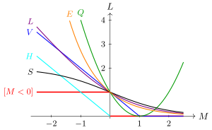
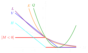
The threshold loss function (red) and its continuous approximations: (SVM), , (logistic), , (sigmoid), (exponential).
Each of these loss functions leads to one method or another, which we have covered one by one in one way or another: here are SVM, logistic regression and even Fisher's linear discriminant. Let us pay attention to the strange loss function of Fisher's linear discriminant. Why is it like this, unlike all the others? It has a right branch that at first sight is altogether unreasonable: it penalises large positive margins. What for? There is one point. When you use the quadratic loss function in Fisher's linear discriminant, remember, there is an additional transformation there: from each object you must subtract the centre of its class. You determine the class centres as parameters and describe each class by a Gaussian, a multivariate one, and it is assumed that the shapes of the Gaussians of all classes are the same: only then does the quadratic discriminant become linear. When you have, as it were, brought all the classes together into one point in order to determine a covariance matrix common to them, at that moment you use such a loss function. It is equivalent to your recovering a Gaussian density in the class, that is, looking at the density of the class from all sides, not only where the boundary between the classes runs but also on the periphery. Hence the right branch.
I am telling this to draw your attention: Fisher's linear discriminant is not very good to use; it is a method considered outdated. But understanding that it has such a loss function leads at once to an idea: can the right branch be zeroed and a smooth loss function used that has a parabola on the left and then zero? It is very similar to the SVM loss function: that one is linear in the left part, and this one will be quadratic. Such a method exists too. It has no selection of support objects, because there is no kink in the loss function, but nevertheless such a modification can be used too, and it is considered a little more advanced than Fisher's discriminant.
Looking at this picture, you should understand that loss functions can be invented however you like; it is not limited to this list. What, for example, is good about the sigmoid loss function? That it is more robust: it does not penalise errors so heavily; you will allow yourself to leave a few more erroneous objects and will not chase them, as the exponential loss function does, which chases objects with an error in order to correct them without fail, as, for example, AdaBoost does. Such is a useful general view of practically all classifiers based on building a separating surface and on the notion of the margin.
The support vector machine
Definition (The support vector machine SVM (two-class)). is the margin in the linear model.
The piecewise-linear loss function:
- The loss function penalises objects for approaching the boundary between the classes.
- The regularisation maximises the gap between the classes and penalises multicollinearity.
The most important properties of SVM:
- a convex programming problem, the solution is unique;
- the solution is sparse: it depends only on the support objects;
- a generalisation to nonlinear models: .
A couple of words about SVM. It is one of the special cases of a margin-based loss function; it has a regulariser, and it has two important properties. The first: we widen the boundary between the classes, the separating strip. And the main thing: the solution comes out sparse, that is, it depends only on part of the objects of the training sample. This is a very important property of SVM: we could in principle throw all the other objects out of the training sample, and the separating surface would come out the same. Thanks to what does this happen? Thanks to the kink in the loss function. In general, if a loss function has a kink, the notion of support objects appears for us, and uninformative objects are discarded. This is an interesting property: when you choose a loss function for your particular problem, see whether you want it to have the property of support objects. What is good about it? That training becomes more stable: since it relies on a subset of objects, adding or modifying some objects of the training sample will not affect the solution much. If you need this property, use loss functions with a kink, as in SVM.
Logistic regression
Definition (Logistic regression (two-class)). The linear classification model . The logarithmic loss function:
The model of the conditional probability:
where is the sigmoid function.
Logistic regression is from the same company; a regulariser can be used in it too, but it has another good property: the margin can be turned into an estimate of the probability of the classes, such a model of the conditional probability used to say with what probability an object belongs to one class or another. In principle, any classifier based on the principle of separability can be turned into a classifier that returns an estimate of the probability of a class; for this there is such a technique as Platt calibration.
Definition (Logistic regression (multiclass)). A linear classifier with an arbitrary number of classes :
The probability that the object belongs to the class :
where translates an arbitrary vector into a normalised vector of a discrete distribution.
Maximisation of the likelihood (log-loss) with regularisation:
And the last point about classification: logistic regression where there are many classes. There we are forced to use a slightly modified function, the : we assign an object to the class for which the scalar product is maximal, and in this way is the direction in which the objects of the class lie. Since logistic regression is a probabilistic model of the posterior probability of the classes, one can use the maximum likelihood principle, the so-called log-loss: the loss function is minus the logarithm of the model of the posterior probability of the classes. And regularisation can be used too.
Loss functions in regression
Now let us run through the loss functions used in regression. The classical case, as we said at the very beginning, is the quadratic loss function. What else is there?
Definition (Quantile regression). The loss function, :
The regression model: linear, .
Reduction to a linear programming problem: the change of variables , ;
The loss function of quantile regression (slide): the penalties for underforecasting and overforecasting differ.
Quantile regression is when the losses from overforecasting and from underforecasting are different for you, and you can measure them. I gave an example in the lectures: forecasting sales volumes when you plan purchases. If you have supplied more goods than needed, they lie on the shelves, and these are small losses. If you have not supplied goods, while there is demand nonetheless, you lose the trade margin, and perhaps even the loyalty of customers, and these are big losses. When we pose this problem as an optimisation problem, it turns out to be equivalent to a linear programming problem. If you ever need to solve problems with such angular loss functions, linear programming is at your service.
Definition (Robust regression). Meshalkin's function: , .
The regression model: .
The formulation of the optimisation problem:
The numerical solution is by the Newton–Raphson method.
Meshalkin's loss function for and the quadratic loss function (slide).
Robust regression is one more way of modifying the loss function, but with a different aim: we do not want objects with large errors to influence the model strongly. When the loss function is quadratic, its branches going off to plus infinity penalise outlier objects very heavily, and this means that the model begins to tune to these outliers as a priority. It would be right to throw these outliers out altogether. In fact this can be done by an iterative process: look at which objects turned out to have anomalously large losses, throw them out and rebuild the model once more. Or one can simply modify the loss function, and then the problem becomes one-pass: the model is tuned in one pass, simply ignoring the outlier objects. One of the ways to set a robust loss function is to give it horizontal asymptotes. It is in effect simply an inverted and shifted Gaussian; one need not even have shifted it.
Definition (SVM regression). The regression model: , , .
The loss function: .
The formulation of the optimisation problem:
It reduces to a convex quadratic programming problem.
The loss function of SVM regression with (red) and the quadratic loss function (blue) (slide).
One more idea about regression: let us not penalise small errors at all. If the answer on an object deviates from the correct one by the amount , our usual residual, in the quadratic loss function it is simply , then here with a positive cut-off is taken: we do not penalise deviations within , being a parameter. The problem is very similar to SVM, and again I draw your attention: the loss function has two kinks, and thanks to this support objects appear. The non-smoothness of the loss function leads to a Karush–Kuhn–Tucker formulation of the problem, additional non-negative variables arise there, and because these variables can vanish, the non-support objects drop out of the formulation of the dual problem. That is how formulations of problems that use loss functions with kinks are arranged.
Regularisation
Regularisers that penalise the complexity of a linear model
We have run through the loss functions; now let us talk about regularisation.
Definition (Regularisers that penalise the complexity of a linear model). A regulariser is an additive addition to the main criterion:
where is the loss function and the regularisation coefficient.
- regularisation (ridge regression, SVM): .
- regularisation (LASSO, Elastic Net, for feature selection): .
- regularisation (Akaike's information criterion AIC, the Bayesian BIC): .
For linear models the typical form of a regulariser is , or . In general a regulariser is usually some penalty for the complexity of the model, for the dimension of the parameter vector; regularisation is simply the number of parameters not equal to zero. Why precisely in linear models? It is in a linear model that the problem of multicollinearity arises: the coefficients at the features can run off to plus or minus infinity. This is a sure sign of multicollinearity, you will have overfitting, and the way to get rid of it is to press the coefficient vector to the origin. This is a technique specific precisely to linear models. In nonlinear models an excessive number of degrees of freedom, an excessive number of parameters, may also lead to overfitting, but it may look not like multicollinearity but some other way. The parameters perhaps also need to be pulled somewhere, but not necessarily to zero: it all depends on how the parameters enter the formula of the model.
Even for linear models there is an amusing special case where the regulariser is a little different. Let us recall compositions: a composition may be a linear composition of some models, simple or weighted voting. Suppose you have built a large number of base algorithms, by boosting, bagging or otherwise, and asked yourself: can the weights of the base algorithms be determined more accurately? You regard the base algorithms as features and build a linear classifier over them; its coefficients are the weights of the base algorithms. What regularisation makes sense here? One of the variants is one that will make the weighted voting as similar as possible to simple voting. For example, you have built bagging, which is simple voting by default, and now decided after all to tune the coefficients a little and make weighted voting out of simple voting. Can overfitting, multicollinearity, arise in doing so? We are building a linear model, after all, so by and large it can. Regularisation is needed, and one can press the coefficient vector to zero, but just as well one can press it to the point where all the coefficients equal one: it corresponds to simple voting. Then the regulariser will be not but . Such is a slightly different situation: a linear classifier is built, but it makes sense to press the coefficient vector not to the zero point but to the vector of ones. That is, this form of regularisation too is not the ultimate truth: situations may arise that will make you look at regularisation differently.
Remark (AIC and BIC). Akaike's and the Bayesian information criteria are mentioned on the slide; they were not in the lectures. They are rather simple modifications of regularisation, and they differ little from each other: they penalise simply the number of parameters used. In the Bayesian information criterion, as far as I remember, the penalty is also multiplied by the logarithm of the length of the training sample, but this is not a very significant correction, because the regulariser is multiplied anyway by the regularisation coefficient, which you choose in one way or another. There are very interesting theories about these information criteria, they were originally derived for regression problems, but I do not include them in the course: it is enough to know about them that they are penalties for the number of parameters of the model.
Non-smooth regularisers for feature selection
Definition (Non-smooth regularisers for feature selection). The general form of the regularisers ( is the selectivity parameter):
Regularisers with the effect of grouping dependent features:
-
Elastic Net: ;
-
Support Features Machine (SFM):
-
Relevance Features Machine (RFM): .
I showed all sorts of non-traditional forms of regularisers. A well-known one is Elastic Net, a weighted sum of and regularisation, and it has interesting properties, in particular the effect of grouping dependent features. Unlike , unlike LASSO, it does not get rid of linearly dependent features so aggressively. If a whole group of features is important for the model, but there are dependences between them, Elastic Net does not strive to throw them all out but strives to equalise the coefficients between them. This happens thanks to the regularisation: the regulariser tries to discard the unnecessary features, but the linearly dependent and nevertheless important features it will try to keep all together, as a group.
There are other ways of aggregating and regularisation: one can make such a gluing, or one can use non-convex regularisers altogether, and they too have their interesting properties. What is good about the Support Features Machine? Elastic Net has this problem: it may keep some noise features too, also grouping them, and will not throw them out of the model. SFM, thanks to aggregating and differently, groups the informative features together and removes the uninformative ones one by one, and the grouping effect does not arise on noise features.
The non-smoothness of the loss function leads to the selection of objects, to the appearance of support objects. The non-smoothness of the regulariser leads to the selection of features. Use non-smooth loss functions and non-smooth regularisers in those problems where you need to arrange such selection: if you want to select both objects and features, then SVM with regularisation or something in that spirit.
Later we will see that regularisers can be much more diverse. The general view of regularisation is probably multi-criteria optimisation. Multiple criteria may also arise in the context of your solving many problems at once, and then they, as it were, act as regularisers for each other. The idea of regularisation begins with very simple things like or regularisation, but then you understand that it is multi-criteria optimisation, and the variety of regularisers that can be used in machine learning is enormous; it is not limited to and . Let me remind you once more: they are natural only for linear models.
Learning to rank
Ranking problems
Definition (Ranking problems (Learning to Rank, LtR, L2R, LETOR)). Ranking is needed wherever a system gives the user a choice from a large number of options:
- the results of a search engine;
- recommendations of books, films, music and other goods;
- recommendations of content in distance education;
- automatic completion of a query (auto-suggest);
- answer options in dialogue systems;
- translation options in machine translation systems.
The criterion is constructed differently in three approaches:
- point-wise (an analogue of regression or classification);
- pair-wise (the quality of pairwise comparisons);
- list-wise (the quality of a ranked list).
Ranking problems were in this semester; you probably still remember them well. We had three approaches, point-wise, pair-wise and list-wise, and they differed precisely in the constructions of the loss functions.
The point-wise approach: ordinal regression
Definition (The point-wise approach: ordinal regression (Ordinal Regression)). The training sample , where .
A ranking function with parameters and thresholds , , :
The loss function is a decreasing function of the margin .
The training criterion by the two nearest thresholds:
The training criterion by all thresholds:
J. D. M. Rennie, N. Srebro. Loss functions for preference levels: regression with discrete ordered labels. IJCAI-2005.
In the point-wise approach a typical example is the so-called ordinal regression. It is a rather old method, and it has many variants; here is one of the fairly recent modifications, from a 2005 paper. You may still have a linear classification model, but here for generality I write that the model is arbitrary, possibly nonlinear, some function of the object with parameters . The main thing is that you get the value of the function ; in classification it is called discriminant, that is, it determines the separating surface, while in this case it in effect ranks the objects. And on the axis of values of this ranking function you place certain thresholds that mark out a finite set of values. This is no classification problem at all; it is more like regression, because on this finite set of values there is an order relation of its own. It is like a scale of marks: how is a student to be given a mark in points for an assignment? We make an algorithm that automatically checks the assignment and gives a mark, say, on a ten-point scale. First it computes a certain score, that is the ranking function, and then it must somehow set the thresholds where 10 points differ from 9, 9 from 8 and so on. These thresholds are also parameters of the model, and we optimise them too.
How are penalties to be introduced, how is the loss function to be constructed? One of the possible ways is from two terms. The object should have fallen into its strip, its correct answer is, say, , and the strip has left and right thresholds beyond which it must not go. There arises, for example, an SVM-like loss function; one could also draw a quadratic one, or some other, depending on what properties we want from the model. Let us set an SVM-type loss function, and we get support objects and the possibility of introducing kernels, as usual in SVM.
The loss function by the two nearest thresholds for an object with (slide).
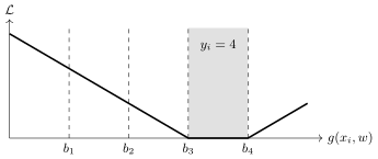
The sum of losses by the two nearest thresholds for an object with (with ): the penalty is zero while falls into the strip , and grows linearly on leaving it across either of its boundaries.
But there is another way of introducing a loss function; it then comes out more broken, piecewise-linear. We penalise not only for the object having left its strip. If it has violated a threshold once, we penalise it, and if it has violated the next threshold too, that is, deviated still further from the correct answer, let us penalise it more strongly. Then there appears a sum over all possible values of from one to : whereas before the loss function consisted of two terms, here it consists of terms. Such is the, in my view, neat construction that arises for ranking problems.
The loss function by all thresholds for an object with (slide).
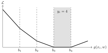
The sum of losses by all thresholds for an object with (with ): each threshold crossed adds its own penalty, so the slope grows with the distance from the correct strip.
The pair-wise approach
Definition (The pair-wise approach to learning to rank). Given: , the training sample; , the correct order on the pairs .
Find: a ranking model such that .
Criterion: the number of wrongly ordered pairs , or the approximated pairwise empirical risk:
where is a decreasing function of the pairwise margin .
The pair-wise approach is a little different. Here the training sample gives not the answers on the objects but the correct order on pairs of objects, and we want to build a ranking model such that it gives on the objects the order that is in the training sample. Let me remind you that the order may be partial. For example, in the problem of ranking search results, the objects are "query–document" pairs, and we can compare only those documents that were found in response to one and the same query; this is one of the special cases of how a partial order arises. Here we construct a pairwise loss function: the sum is now not over individual objects but over pairs of objects. And we can apply the same ideology as in classification: define a margin, but a pairwise one too. It is the difference of the values of the model on a pair of objects, and if this difference is negative, it means we have made an error with the order between these objects; they have to be swapped in the ranked list. For their being wrongly ordered, a penalty. This is the standard way of adapting margin-based approaches from classification to solving ranking problems.
I can also remind you at this point that the criterion, the sum over all pairs, is the number of wrongly ordered pairs of the sample. If the order is linear and we are also solving two-class classification, that is, we have only two possible answers on the objects, then this criterion is something like one minus AUC. More precisely, to get AUC from this criterion, it must first be normalised, divided by the cardinality of one class and by the cardinality of the other class, then the criterion is normalised into , and one says that this criterion is minimised and AUC is maximised. AUC is one minus the normalised criterion. An interesting link results between things that at first sight may not be linked in one's head: explicit maximisation of AUC with such an approximation of the loss function is nothing other than the pair-wise method of solving the ranking problem. This too is useful to realise. If you have a classification problem and the client says: "I need AUC maximised", what does that actually mean? It is actually a ranking problem, and it can be solved by the same methods as ranking problems usually are.
A list-wise approach based on the pair-wise one
Definition (A list-wise approach based on the pair-wise one). The stochastic gradient method for the pairwise criterion:
is a non-smooth criterion computed on a list of objects ranked in decreasing order of the values . Examples of non-smooth criteria : MAP, NDCG, pFound and others.
is the change of when are swapped in the list.
LambdaRank: multiplying the gradient by leads to approximate optimisation of the non-smooth criterion :
C. Burges. From RankNet to LambdaRank to LambdaMART: an overview. 2010.
And one more reminder. I will not go into how list-wise approaches to ranking are arranged; the main thing worth remembering: there is a heap of non-smooth criteria, MAP, NDCG, pFound, and a heap more have been invented. They are all based on our re-ranking our sample with the ranking function and looking where in the list the relevant objects are. Criteria of this kind are all non-differentiable; they are very hard to optimise directly. The LambdaRank method is based on the fact that pairwise methods are very easily adapted for optimising list-wise functionals. It is a rather unexpected solution, but very simple at that, described in this 2010 paper. You use exactly the same stochastic gradient method as for the pairwise criterion, but multiply the gradient step by , by how your complex non-differentiable criterion will change when the pair of objects and is swapped in the ranked list. This amusing modification shows that even if your criterion is very complexly arranged, as in the ranking problem, it can be approximately optimised by simpler criteria based simply on pairwise comparisons.
This too is a story about how to set a criterion. One can clutch one's head and say: "Oh, it is terrible", and then it turns out that instead of it one can optimise a slightly different criterion, a much simpler one, and build a small correction into the optimisation method. Probably this idea may still hit the mark somewhere else; where, to be honest, I do not know, but the idea is well worth putting into your piggy bank of ideas about machine learning.
Unsupervised learning
Estimating a probability density
The very first and probably the most important problem of unsupervised learning that comes to mind is estimating a probability density. It seems to me even more fundamental than the clustering problem, which also comes to mind first when unsupervised learning is mentioned.
Definition (The problem of estimating a probability density). Given: a training sample .
Find: the parameter vector in the model .
Criterion: the maximum likelihood
or the maximum a posteriori probability
where is the vector of hyperparameters of the prior distribution.
Here you consider a sample and assume that it was generated by some probability distribution, and that the elements of the sample are independent; this has to be assumed, otherwise you will not get a sum of logarithms. You build a parametric model and determine its parameters from the maximum likelihood principle. The loss function here is minus the logarithm of the probabilistic model: minus because you maximise the likelihood, while when people talk about losses it is a minimisation problem. If you have some prior assumption about the parameters of the model , you can formalise it as a prior distribution and use the maximum a posteriori probability principle. Then what is the logarithm of the prior distribution? It is regularisation. That is the probabilistic meaning of a regulariser. Even the regularisers we considered, and , can be given a probabilistic meaning too. In linear models of regression and classification you impose constraints on the parameters of the model and say: let the parameters be concentrated in the neighbourhood of zero, that is, the prior distribution has its expectation at zero. If it is Gaussian, that is the regulariser; if Laplacian, the regulariser.
In regression and classification problems the loss function too can be given a probabilistic meaning. One can say that in fact we have some model of given , there are errors, they are distributed somehow, and the logarithm of the density of this distribution is the loss function. That is, one can easily pass from probabilistic formulations of problems, where a probabilistic model of the data is built and the maximum likelihood principle is used, to problems where you simply formalise the form of the model and then set the form of the criterion. Very often these two views are equivalent, and you can reason either in probabilistic terms or in non-probabilistic ones. For example, you build a separating surface and set a loss function, and then it turns out that this is equivalent to modelling the posterior probability of the classes.
Estimating a mixture of densities
Definition (The problem of estimating a mixture of probability densities). Given: a training sample .
Find: the parameters , in the model .
Criterion: the maximum likelihood
or the maximum a posteriori probability
where is the vector of hyperparameters of the prior distribution.
If one parametric model does not allow the problem to be solved well, for example you cannot describe well by a Gaussian a distribution that is not unimodal, that is, where the objects concentrate not around one point but around several, then it makes sense to use mixtures. A mixture is also a parametric probabilistic model, a two-level one. It assumes that you first toss a many-sided asymmetric coin and determine from which mixture component your object will be generated: is the probability of the mixture component. And then from this component you generate the object itself. It is a two-stage generative model, and we are solving the inverse problem: we are given a sample, and we want to understand by what components it was generated and what the probabilities of these components were. Sometimes the problem is also posed of understanding how many components there were; that is already a problem of structural modelling. We can solve the problem with a fixed number of components and then vary it somehow, or we can devise an algorithm that itself creates and removes components and in the end converges to some number of them.
Here one can apply the same criterion of maximum likelihood or maximum a posteriori probability, and the EM algorithm arises, the splitting of a mixture of distributions. You first estimate with what probability each object is generated by each component, these are the so-called hidden variables, and then with their help you solve the maximum likelihood problems for each mixture component separately. This scheme is fairly general: wherever you solve non-trivial problems of building probabilistic models of data generation and understand that your data are so complex that they are described only by a probabilistic mixture, a rather cumbersome model, welcome to the kingdom of the EM algorithm; it will help you.
Clustering
Definition (The clustering problem). Given: a training sample .
Find:
- the cluster centres , ;
- which cluster each object belongs to, .
Criterion: the minimum of the intra-cluster distances
in the case of the Euclidean metric .
Clustering is a similar problem. Why similar? This formulation, it would seem, is classical: there is the -means method, which solves this optimisation problem; it is also called Lloyd's algorithm. In fact this is nothing other than also a certain probabilistic assumption that the classes are, first, spherical, second, Gaussian, and third, their number is given and fixed. In such a case the problem of splitting a mixture of spherical Gaussians, each Gaussian set by the position of its centre and its variance, with fixed variance turns exactly into this formulation. That is, one can say that the classical clustering problem for the -means method is the most primitive variant of the problem of separating a mixture of Gaussians: Gaussians not only with diagonal covariance matrices, but with the same variance on the diagonal, and a constant one at that. Simply spherical clusters with fixed radii, the same for all clusters. Such is an amusing understanding of what the -means method really is: a representation of the data by a set of spherical Gaussians. How well does such a representation suit you for solving your particular problem? If your clusters have very different diameters, that is, variances, if they are not spherical but elongated, is it worth using the -means method?
On the other hand, a probabilistic mixture, and specifically a mixture of Gaussians, is a universal approximator of densities. Just as there are universal approximators of functions, the Fourier expansion or representation by polynomials, so for distributions there are universal approximators of their own, and a mixture of Gaussians is one of them. Even if your classes are of some complex elongated shapes, can you really not cover them with balls? Of course you can. It will be such a clustering by balls, and that is exactly the problem the -means method solves: it determines at once both the cluster centres and the membership of each object in a cluster, being the number of the cluster to which the object belongs.
This is also called hard clustering. The previous problem, separating a mixture of distributions, is soft clustering: there you learn the probability with which each object belongs to each mixture component , that is, each object will have a vector of probabilities as a by-product of this problem. From soft clustering it is always very easy to make hard clustering: apply and say that the object belongs to the component to which it belongs with the maximal probability. But the -means method is by the very formulation of the problem hard clustering; soft clustering can no longer be made from it. This again is a story about how, by the very formulation of the optimisation problem, by the loss functions, to fix some properties of the model and the solution. Whether you need hard clustering or soft comes from the problem, and then you understand which of these approaches it makes sense to use.
The one-class SVM
And here is a small piece I did not tell you in the course: it somehow dropped out and did not fit with anything. You probably know, I mentioned it, and it is written in many places, that SVM was proposed in the early 90s under the name support vector machine; it was invented by Vladimir Naumovich Vapnik after he had moved to the USA. But in fact this method was created here at the end of the sixties and the beginning of the seventies and was called the generalised portrait method; it was made together with Alexey Yakovlevich Chervonenkis, by a whole team; they had a whole scientific school. An amusing fact: when they were just beginning to develop the generalised portrait method, one of the first problems they solved was precisely this one-class SVM.
Definition (The one-class SVM (OSVM)). Given: a training sample .
Find: the centre and the radius of a ball enclosing the whole sample except the anomalous outlier objects.
Criterion: minimising the radius of the ball and the sum of penalties for leaving the ball:
With the properties of the solution are analogous to SVM:
- a convex quadratic programming problem;
- the solution is sparse: it depends only on the support objects;
- a generalisation to nonlinear models: .
The one-class SVM (slide).
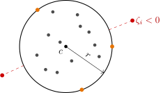
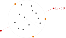
The one-class SVM (a schematic): a ball with centre and radius ; the orange objects on the boundary are support objects, the red ones outside the ball are outliers.
The problem is posed as follows. You have a sample of points, and you want to describe it by a ball: determine the centre and radius of the ball so that it is as compact as possible, we will minimise the radius, and so that it encloses, preferably, all the points of the sample. But if there are points in the sample that lie too far away, let them be considered outliers. That is, it is a way of detecting atypical objects: a typical one is when we are not far from the centre of the ball, and if a point has flown off too far, it is already an outlier object. It is a way of filtering out outliers.
How is the problem posed? We minimise, first, the square of the radius, and second, penalise the outliers for being at a distance greater than the radius. How is this done? Again take a decreasing function of the margin; the margin here is the difference of the square of the radius and the square of the distance from the point to the centre of the ball. If we take a piecewise-linear loss function, as in SVM, the main thing being that it has a kink, then exactly as in SVM a convex quadratic programming problem arises. It will have a unique solution, this solution will be sparse, support vectors will arise. Moreover, one can generalise to nonlinear models by replacing the scalar product by a kernel. That is, the whole story repeats exactly as in SVM, although the formulation of the problem, look, is different. And what is neat here: passing to a kernel allows the sample to be described not only by a ball but by any surfaces at all. Take a polynomial kernel, or a radial basis one, or a neural network one, anything that is a kernel, and you will have a really neat way of outlining the sample by some surface so that it encloses almost the whole sample, except perhaps a small number of outliers. This is such an approach to outlier detection: one can call it the one-class SVM, or outlier detection.
Remark (Where one-class classification is applied). It is outlier detection: before you is a sample, for example not labelled at all, and atypical objects have to be found. An example is fraud detection. You watch the transactions of the clients of a bank or some service where financial or some other fraud is in principle possible. I have also been told about applications in online computer games, where a large number of people play: fraudsters appear there who try to get round the rules of the game and get some additional goodies, and they are fought in roughly the same way as banks fight fraudsters. The problem may be simply detecting atypical behaviour: honest players behave in a certain way, while those who cheat have some unusual patterns of behaviour, and we do not know which. It is good if we are experts, understand what fraud schemes there are, and write out models of frauds directly. But that is a hard path, because fraudsters keep inventing new schemes, and we have to chase them, build and build new models. So the approach is this: without a labelled sample, without knowing at all what fraud there is, let us simply single out something atypical, and then perhaps look at it with our eyes and understand whether it is fraud or simply an unusual but within-the-rules way of behaviour of a client. Or detecting attacks in computer networks: you do not know in advance what attacks are being prepared, and the preparation of an attack may be carried on long in advance, by some users who have illegally gained access and begun to do something unusual. Detecting such users is also such a problem.
Semi-supervised learning
Semi-supervised learning and the transductive SVM
We will little by little extend the formulations of problems. One more problem I want to recall is semi-supervised learning. It is a problem where you have many unlabelled objects and unsupervised learning should, as it were, work, but there is a small group of objects that are labelled after all; they are not enough to build a full-fledged model. The idea arises of combining somehow the information about the labelled objects, of which there are as a rule few, and the information about the unlabelled ones. On the unlabelled ones something like clustering has to be done, on the labelled ones something like classification, but at the same time all objects have to be classified, both labelled and unlabelled.
Definition (The semi-supervised learning problem (SSL)). Given:
- , labelled objects (labeled data), ;
- , unlabelled objects (unlabeled data).
Find: the classifications of the unlabelled objects.
A criterion without a classification model (transductive learning):
When building a classification model, :
Here precisely the view of a machine learning problem as a problem with regularisation helps, and it can be understood in two ways. It is even unclear whether to consider these as separate loss functions: on the labelled objects their own loss functions, on the unlabelled their own. Here are two different examples. The first is called transductive learning, because we do not use a model at all: we simply want to label the unlabelled objects, and for this we introduce such a criterion, as in clustering. But if we want to build a classification model that has its own parameters , and tune them, a sum of two criteria appears again. One can look at this in different ways; these are only words, and they do not affect the solution of the optimisation problems in any way: one can interpret one functional as the main one and the second as its regulariser, or one can say that on different objects we simply have different loss functions.
Definition (The TSVM method, the transductive SVM). is the margin of the object .
- The loss function penalises a decrease of the margin.
- The loss function penalises an object for falling inside the separating strip.
Training the weights , on a partially labelled sample:
The loss functions of the transductive SVM (slide).
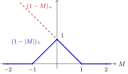
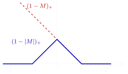
The loss functions of the transductive SVM: for labelled objects penalises a decrease of the margin; for unlabelled ones does not depend on the label and penalises an object for falling inside the separating strip .
As an example, the transductive SVM, when you penalise objects for falling into the separating strip between the classes. You want to make the separating strip not only as wide as possible but also with as few objects in it as possible, that is, as it were, do a clustering. Such a loss function arises; it too is piecewise-linear, support vectors arise too, kernels arise too, and then this whole story is as in SVM.
PU-learning
And here is one more little problem I did not mention. It is a little like the one-class one, but the situation of application is different, and the technique usually used, a very simple one, is different too. PU-learning is in fact a rather serious topic, because it has many different applications; below I give two surveys, one old, the other new. People really do work actively on this problem and try all sorts of different methods, but, strangely enough, one of the best is the simplest solution.
Definition (A special case of SSL: PU-learning (Positive and Unlabeled)). Examples of problems where objects of only one class are known:
- detecting fraudulent transactions;
- recommender systems, personalisation of advertising;
- medical diagnosis with an unknown history;
- automatic filling of a knowledge base with facts.
A model of two-class classification . The unlabelled ones are treated as negative with weight :
One of the successful methods is Biased SVM.
Gang Li. A Survey on Positive and Unlabelled Learning. 2013. J. Bekker, J. Davis. Learning From Positive and Unlabeled Data: A Survey. 2020.
The problem is that we have a labelled sample, but it contains objects of only one class. Let me give an example from my own practice of twenty years ago. On a currency exchange we were solving a problem of financial supervision. Experts who sit and monitor the market have to catch cases of unfair trading: insider trading, price manipulation and other not very good things that market participants sometimes do. Of course, one wants to build a rule that detects all this bad activity in trading. But what is the trouble? We have cases where such activity was detected; there are not very many of them, and obviously the experts who sit and catch such things certainly have not caught all of them, since it is manual work. In principle these cases make up the training sample, but it contains only examples of anomalous behaviour, those we consider fraudulent actions, unfair trading. How is everything else to be formed, what we do not consider fraud? If we are catching fraudsters, then for us this is the class , positive, and the negative one is ordinary trading operations; there is a huge majority of them there, 99.99 per cent; there are few fraudsters, and few fraudulent operations. How is a training sample to be formed if experts have labelled only objects of the class , and there are in principle no objects of the class ?
Then they are generated somehow: these are simply situations that are with high probability normal, simply the whole prehistory of the data. And in such a case we make a weighted loss function: the objects of the class go with some large weight, and the synthesised objects, which we by default consider objects of the class , with a smaller weight. There are many of them, but they are unreliable, because nobody has confirmed by hand that these really are not fraudulent actions. And, strangely enough, this is one of the most successful methods, and it is the simplest, although a huge number of different heuristics have been invented for PU-learning. From time to time works appear that show that this problem should be solved in a much more complicated way, but practice shows that one need not make a big fuss: PU-learning is not such a hard problem.
These are probably the two new points of today's lecture: one-class classification and PU-learning.
Representation learning
Next, a few sketches on the topic of the recent past, the middle of this semester, where we considered various vector representations. As a rule, these too are unsupervised learning problems.
Matrix factorisations
Definition (The problems of low-rank matrix factorisation).
- Dimensionality reduction for classification or regression.
- Forming vector representations of objects.
- Filling in missing values in a matrix.
Given: a matrix , .
Find: matrices and such that
Why classical SVD is abandoned in practice:
- a non-quadratic loss function ;
- nonnegative matrix factorisation: , ;
- sparse data: ;
- orthogonality is not needed or not interpretable.
Let us begin with problems of low-rank matrix factorisation, when you have some matrix, usually with missing values, and you have to fill in these gaps. By the way, this is a self-sufficient problem, and once, several decades ago, it was considered a separate machine learning problem; now it has become routine. Rather rarely are such methods applied in which, before solving a classification or regression problem on an "objects–features" matrix that has gaps, you pose an intermediate problem of preprocessing the data: let us fill in these gaps. For example, each feature in turn is regarded as the target, and a regression problem is solved: from all the other features we try to predict this feature and in this way fill in the gaps. Such methods are used less and less; matrix factorisation methods are used more often. Our matrix , which is known not in all cells but only in some subset , we try to approximate by a low-rank matrix factorisation, the product of two matrices whose intermediate dimension is substantially smaller than and substantially smaller than . This can be done in different ways, but classical SVD is precisely useless here, because it assumes that the matrix is completely filled. But there are many methods of solving such problems where the sum is taken only over the filled cells.
Autoencoders
A close formulation of the problem is autoencoders. In fact there is a close connection between matrix factorisation problems and autoencoders: autoencoders are in effect a good nonlinear generalisation of matrix factorisation problems.
Definition (The problem of building an autoencoder (unsupervised learning)).
- , the training sample;
- , the encoder, the code vector ;
- , the decoder, the reconstruction .
The superposition must restore the original :
The quadratic loss function: .
Example 1. The linear autoencoder: , ,
Example 2. A two-layer network with activation functions , :
We are given a sample, and we want to synthesise for each object a vector representation that preserves the maximum of information about this object. The original object may be given in some complicated way: with missing data, with non-numerical data at all, as a graph, God knows what else. Nevertheless we want to make a vector out of it. In effect the encoder is a synthesiser of the vector representation of an object; one can also look at this problem as feature generation, a way of generating features. The encoder makes a code vector out of the object . But to preserve the information about the object in the vector as fully as possible, we must pose the problem of the possibility of decoding, of getting the vector back from the code vector with maximal accuracy. So we build such a superposition and say that it must restore the original objects, and we measure the accuracy of restoration by some loss function, we have discussed a heap of them today already, for example as in the method of least squares.
Where are our matrix factorisations here? It turns out that if we take a linear transformation as , and as too, where and are simply matrices that multiply vectors from the left, this will be nothing other than a matrix factorisation. The optimisation problem, where the loss function is quadratic and the encoder and decoder are linear, simply turns into the matrix factorisation problem as a special case. And in autoencoders we are entitled to make the encoder and decoder more complex, up to neural networks, up to deep ones. Clearly this is a much richer model, which can solve much more complex problems than simply matrix factorisation.
Definition (Autoencoders for supervised learning). Data: labelled , unlabelled .
Joint training of the encoder , the decoder and a predictive model (classification, regression or other):
where is the encoder, the decoder, the predictor; the loss functions: , the reconstruction, , the prediction.
Dor Bank, Noam Koenigstein, Raja Giryes. Autoencoders. 2020.
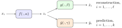
An autoencoder and a predictive model with a common encoder (a schematic): the reconstruction with losses is trained on all objects, the prediction with losses on the labelled ones, and both problems tune the common parameters of the encoder .
The next very important concept about autoencoders: one and the same vector representation can be used to solve several problems at once. The encoder makes a code vector from an object. First, we force this vector to be as informative as possible: we build a decoder and force the reconstruction to be similar to the original object; in this way we ensure the informativeness of the vector representations . And the vector representations themselves we need in order to solve some machine learning problem where the objects must be represented by vectors: regression, classification, anything at all. And we solve two problems at once. It may well be that we have a sample of unlabelled objects and labelled ones: on the labelled ones we want to solve a classification problem, and on the combined sample a reconstruction problem; we want to reconstruct all objects, both labelled and unlabelled. We tune all the parameters at once: , the parameters of the encoder, , of the decoder, , of our predictor.
Here, of course, there is a question: who is whose regulariser? Or simply consider it as two problems that we solve at once, but which have a common vector representation , and the parameter is tuned so that both problems are solved well. This is already an element of multi-task learning, and such problems arise more and more in modern machine learning; you will surely have to face them one way or another. Why do they arise more and more often? Because we increasingly speak not simply of machine learning but of artificial intelligence. One of the interpretations of the difference: artificial intelligence is able to solve a broader class of problems where the original objects are complexly arranged, complexly structured, in some raw representation. Our course was almost entirely about how to solve problems with objects that are vectors; and if an object is complexly arranged, it still has to be turned into a vector, and this can be done by one encoder or another.
Multidimensional scaling and graph factorisations
Definition (Multidimensional scaling (MDS)). Given: , a sample of edges of a graph ; , the distances between the vertices of the edge .
Find: vector representations of the vertices , so that vertices close (in the graph) have close vectors.
The stress criterion:
where is usually the Euclidean distance, are weights (which distances matter more: large or small).
It is usually solved by the stochastic gradient method (SG).
With the sample is projected onto the plane:
- it is used to visualise cluster structures;
- the shape of the point cloud can be tuned by the weights and the metric;
- the drawback: distortions are inevitable;
- the most popular method for visualisation is t-SNE.
I. Chami et al. Machine learning on graphs: a model and comprehensive taxonomy. 2020. Laurens van der Maaten, Geoffrey Hinton. Visualizing data using t-SNE. 2008.
One more example of an encoder is multidimensional scaling, where information about the distances between objects is given, and you have to synthesise vector representations of these objects. What is it used for? For example, to get vector descriptions of objects in a two-dimensional space and simply display them on a graph: project a multidimensional metric space, where objects and the pairwise distances between them are given, onto the Euclidean plane and show what it looks like. I will not go into what methods there are; I told about t-SNE.
Definition (Graph (matrix) factorisations (graph factorization)). Given: , a sample of edges of a graph ; , the proximity between the vertices of the edge , for example , the adjacency matrix of the vertices.
Find: vector representations of the vertices, so that vertices close (in the graph) have close vectors.
The criterion for an undirected graph ( is symmetric):
The criterion for a directed graph ( is non-symmetric):
It is usually solved by the stochastic gradient method (SG).
I. Chami et al. Machine learning on graphs: a model and comprehensive taxonomy. 2020.
A slightly different way of building is when we approximate not distances but proximities, and proximities can be approximated by scalar products of the vector descriptions of the objects. This is one more encoder, and it is pleasant in that it is very similar to a matrix factorisation; it is one. It would seem that we are given a graph, and its edges display some information about the proximity of objects, but in fact we have not gone anywhere from the matrix factorisation of a given matrix. Very many such situations arise where about the objects we may know, first, some information about the object itself, some vector or perhaps more complexly structured information, and second, information about the interactions between the objects; then something like an adjacency or proximity matrix arises. This often occurs in practice, and we still want to build a single vector representation of an object that would encode in itself both the links of this object with other objects and the information about the object itself. Such problems too are becoming more and more numerous.
Definition (GraphEDM: a generalised autoencoder on graphs). The Graph Encoder Decoder Model generalises more than 30 models:
- , the input data about the edges;
- , the input data about the vertices, feature descriptions;
- , the vector representations of the vertices of the graph;
- , the decoder that reconstructs the data about the edges;
- , the decoder that solves the supervised problem;
- , (semi-)supervised data about the vertices or the edges;
- , loss functions.
I. Chami et al. Machine learning on graphs: a model and comprehensive taxonomy. 2020.
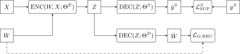
The generalised autoencoder on graphs GraphEDM. The encoder builds the vector representations of the vertices from the data about the edges and about the vertices ; one decoder solves a supervised problem, and its output is compared with the labels ; the other reconstructs the data about the edges, and its output is compared with the original (dashed).
I also showed you this scheme when we talked about vector representations of graphs. It is a 2020 survey that I liked very much, machine learning on graphs. I liked it because the authors proposed such a general scheme; let it look somewhat excessively generalised, but it really does generalise several dozen models, exactly what I was talking about. There are certain objects that sit in the vertices of a graph; there is information about these objects and information about the edges, that is, about the links between the objects. We build an encoder that turns all this information into vector representations of the objects. For these vector representations to be good, we must, first, build a decoder, ensure the reconstruction of the information about the edges of the graph, and second, ensure the solution of some applied problem we need on these objects.
For example, the problem of financial monitoring. There are companies about which there is some information; there are bank transactions between these companies; some of the transactions are suspicious, and there is information about that too. This is a typical example that fits the general scheme. We need to get a vector description of the companies that have to be checked. Tens of thousands of companies across the country: we cannot go to each with inspections, but we can solve the problem of which companies to send for inspection with priority. Vector representations of such objects allow scoring to be done: knowing that some companies engage in illegal activity, and having formed such a training sample, we can already build the supervised part of our criterion. And for the vector representations to be as informative as possible, that is, to reflect the behaviour of a company, we build a reconstructor of links that tries to predict the company's transactions. More and more such applications appear, because machine learning comes into fields where objects can be very complexly arranged, or where there is a whole environment of interacting objects. And here again there are two different loss functions: one for reconstruction, the other for solving the supervised problem, and there may be a dozen more supervised problems there. A scheme arises in which multi-task learning is used: many problems are solved on the same vector representations. Representation learning and autoencoders: this is a general umbrella name for a whole heap of methods where we learn representations of objects.
Non-classical learning paradigms
Transfer learning
Next, various non-classical learning paradigms, where again there is a play with loss functions. This repeats one of our lectures practically word for word, so I will run through it briefly.
Definition (A deep convolutional network as a way of vectorising images). The layers of a convolutional network gradually simplify the structure of an image and increase the dimension of the feature vector: the explicit structure of the image turns into a feature vector, and the last layer solves the classification problem.
Yu. V. Vizilter, V. S. Gorbatsevich. Structural-functional analysis and synthesis of deep convolutional neural networks. MMPR-2017 (in Russian).
Deep neural networks are in effect also a way of learning vector representations, embeddings. For example, when there is an image at the input, convolutional networks gradually increase the dimension of the vector in each pixel but reduce the size of the picture, in the end contracting it to one, and we get a vector representation of the whole picture. Then we train this vector representation so that it solves the problem of recognising objects in images well, if we talk, for example, about the ImageNet competition.
Definition (Pre-training of neural networks). A convolutional network for image processing:
- , convolutional layers for vectorising objects;
- , fully connected layers for a particular problem.
The convolutional layers trained on a large labelled sample (for example, ImageNet) are used to obtain features, and on the target data only a classifier over them is trained (for example, SVM).
Jason Yosinski, Jeff Clune, Yoshua Bengio, Hod Lipson. How transferable are features in deep neural networks? 2014.
Definition (Transfer learning).
- , the universal part of the model (vectorisation);
- , the problem-specific part of the model.
The base problem on the sample with the loss function :
The target problem on another sample , with other , :
With this may be much better than
Sinno Jialin Pan, Qiang Yang. A Survey on Transfer Learning. 2009.
With this story one can do, for example, this: cut off the vector representation trained on ImageNet and, instead of the problem of classifying objects in a picture, solve some other problem. This is called transfer learning: we have trained vector representations of objects on one problem, on some gigantic training sample of the ImageNet type, and then we solve the target problem on a small sample, but our vector representations are already trained.
Multi-task learning
Definition (Multi-task learning).
- , the universal part of the model (vectorisation);
- , the specific part of the model for the task .
Simultaneous training of the model on the tasks , :
Learnability: the quality of solving an individual task improves as the sample size grows.
Learning to learn: the quality of solving each of the tasks improves as both and the total number of tasks grow.
Few-shot learning: to solve the task a small number of examples is enough, sometimes even one.
M. Crawshaw. Multi-task learning with deep neural networks: a survey. 2020. Y. Wang et al. Generalizing from a few examples: a survey on few-shot learning. 2020.
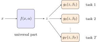
Multi-task learning (a schematic): the universal vectorisation is trained on all tasks at once, and each task has its own specific part with its own parameters . Transfer learning is a special case: is trained on a big task and fixed, and for a new task only its is trained.
A generalisation of this approach is multi-task learning, which I have already mentioned today: we solve many tasks; they are indexed here by the index . For each task there is a specific part of the model, and there is a part universal for all tasks, for example the one that builds vector representations of objects. The objects may be images, but of the most diverse kinds: in one task kittens and puppies, in another cars, in a third Chinese characters and so on. And we want to train a universal vector representation that is able to tell us something informative about any image.
Self-supervised learning
Definition (Self-supervised learning). The vectorisation model is trained to predict the relative position of pairs of fragments of one image (8 possible positions of the second fragment relative to the first).
The advantage: the network learns vector representations of objects without a labelled training sample (without ImageNet).
Carl Doersch, Abhinav Gupta, Alexei A. Efros. Unsupervised visual representation learning by context prediction. ICCV 2015.
And one more special case is self-supervised learning, also a very interesting model. Instead of collecting a training sample, for example ImageNet, we take an unlabelled sample and invent an artificial problem that we can solve: for example, determine how small fragments are located relative to each other in an image. To solve this problem we too will have to create an encoder, that is, a model for vectorising an image. And it turns out that with such training this encoder is in no way worse than one trained on ImageNet, where there are 15 million labelled photographs and enormous human labour has been invested. Several years later it turned out that this human labour need not have been invested, and one could have solved such a problem at once. But who knew; the ways of research are inscrutable.
Distillation and privileged information
A couple more examples on similar topics, where there is a play with both samples and loss functions.
Definition (Model distillation, or surrogate modelling). Training a complex model , "long and expensive":
Training a simple model , possibly on other data:
Examples of problems:
- replacing a complex model (climate, aerodynamics, etc.) that is computed on a supercomputer for months by a "light" approximating surrogate model;
- replacing a complex neural network that is trained for weeks on big data by a "light" approximating neural network with a minimised number of neurons and connections.
Here we train a simple model from a complex one, that is, the complex model acts as a teacher. It was trained long and expensively, or it was some complex computational process that worked for half a year on supercomputers to model some phenomenon. And we want to make a surrogate model, for example to stretch a neural network over this complex model so that it works practically no worse: having lost half a per cent of quality, we gain greatly in efficiency, in the sense of being able to compute this model.
Definition (The problem of learning using privileged information). is information about the object available only in training.
Separate training of the student model and the teacher model:
The student model is trained to repeat the errors of the teacher model:
Joint training of the student model and the teacher model:
D. Lopez-Paz, L. Bottou, B. Schölkopf, V. Vapnik. Unifying distillation and privileged information. 2016.
A similar situation is privileged learning: here too one model learns from another. The difference is that the teacher model has access to certain privileged information, a description of the object that is available only at the training stage. The student will have to be able to solve the problem when there is no access to such information. This problem too has very many applications. For example, we label texts in order to single out some non-trivial fragments, say a positive or negative sentiment regarding some aspect. We do not simply say that the author of this review regards this model of telephone well, but single out in the text the fragment because of which we say so. That is, the expert does a more detailed labelling. But when we need to single out aspects and their sentiments in real texts, nobody will single out these fragments for us: we must build a method that will learn to single out these fragments itself, and it will train on the singled-out fragments. Here is an example of a situation where privileged learning can be applied. In its structure it is in fact very similar to distillation or surrogate modelling: here too a simpler model is trained from a more complex one; only the situation is somewhat different. Either the complex model was trained long and expensively on a separate sample, or the complex model was trained in the presence of some additional information.
Variants of problem formulations in terms of data (slide): the training part (top) and the test part (bottom); are the features, the answers, the privileged information, available only in training. V. Vapnik, A. Vashist. A new learning paradigm: Learning Using Privileged Information. Neural Networks, 2009.
In this picture one can see all the possible schemes: supervised, unsupervised, semi-supervised, transductive learning. Red marks where there is no training information. Privileged learning too can be both supervised and semi-supervised, but it differs in the presence of the matrix , additional information about the training objects, which is absent on the test objects. That is, the student model will have no right to use the privileged information, but nevertheless must somehow learn to repeat after the teacher both the correct answers and the teacher's errors, it will inevitably reproduce them, but nevertheless it will work better than a model that was trained on alone.
Generative adversarial networks
Definition (A generative adversarial network (Generative Adversarial Net)). The generator learns to produce objects from noise . The discriminator learns to tell them from real objects.
Given: a sample of objects from .
Find:
- a probabilistic generative model : ;
- a probabilistic discriminative model .
Criterion: training the discriminative model :
training the generative model on random noise :
Ian Goodfellow et al. Generative Adversarial Nets. 2014.
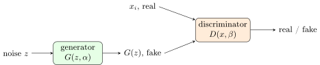
A generative adversarial network (a schematic): the generator turns a random vector into an object, the discriminator learns to tell the real objects of the sample from the generated ones, and the generator learns to deceive it.
And the last situation where there is a play with different loss functions is, of course, generative adversarial networks, GAN. We build two models at once. One model learns to produce some very complexly arranged objects, for example images; the second learns to tell the produced, fake objects from real ones. And they in effect play a minimax game. One and the same functional is introduced, the quality functional of the discriminator. We train the discriminator so as to maximise this functional, and the generator, on the contrary, learns to minimise it over its parameter ; the first term then drops out, because it does not depend on . That is, it is one and the same functional: the discriminator learns to maximise it, and the generator to minimise it. I showed well-known examples of GANs in the lectures.
In this concluding part we have run through those formulations of problems that can be considered the most recent, the most modern, and which really do arise more and more often in practice. Precisely because in practice we begin to work with complexly structured objects that require either multi-task learning or a separate trainable vectorisation, as happens with images or with graphs; problems on graphs appear more and more. Remember this scheme: it may well be useful to you in practice. It seems to me that these are precisely the things that will most likely arise in the coming years in various difficult problems. All these techniques, playing with different models, with different loss functions, with different regularisers, are probably the quintessence of machine learning today. We have long moved away from the simple regression and classification problems with which we began today. Speaking now of artificial intelligence, we are aimed at solving problems where there is usually an element of trainable vectorisation, an element of multi-task learning, some non-trivial regularisers, or even several at once.
Instead of a summary: a typology of machine learning problems
- Data preparation: feature extraction, feature selection, missing values, outlier detection.
- Supervised learning: classification, regression, learning to rank, forecasting.
- Unsupervised learning: clustering, association rule learning, density estimation, one-class classification (anomaly detection).
- Semi-supervised learning: transductive learning, learning from positive examples (PU-learning).
- Representation learning: feature learning, matrix factorization, manifold learning.
- Deep learning.
- Similarity and relational learning (similarity/relational learning).
- Learning the structure of the model (structure learning).
- Privileged learning (privileged learning, distilling).
- Adversarial learning.
- Dynamic learning (online/incremental learning).
- Active learning.
- Reinforcement learning.
- Transfer learning.
- Multi-task learning (multitask learning).
- Meta-learning (meta-learning, AutoML).
Instead of a summary, here is such a little list, in which I have tried to generalise what problems machine learning consists of at all; I tried not to miss anything. In red on the slide I marked what we mentioned today, although there was more in the course: for example, there were incremental and active learning and reinforcement learning in the course, but today, I am sorry, we did not get round to them. And about similarity learning we also said little in the course: in effect there was one episode, when we looked at the problem of how to learn a metric. By the way, remember which episode in the whole course we had when we were learning metrics? A little test question on understanding the course. It was the Siamese network DSSM applied to the ranking problem, where we measured the distance between the text of the query and the text of the document, and both were vectorised by one and the same neural network, which is why it is Siamese. We train the network at once so that it vectorises both queries and documents well, and then compare their vector representations and tune them on click data. But of course similarity learning is a more extensive topic; it would have been worth touching on more deeply; one cannot cram everything into one course.
Remark (BERT or topic models). If we want to get embeddings of a text collection, what is preferable now, topic models or neural network models like BERT? It all depends on the problem. How is BERT better than topic modelling? First of all, in being a deep neural network, that is, a very complex nonlinear transformation. The transformer, and BERT in particular, is tuned on huge training samples, it is said of it that it has seen everything in the language, and it is given the task of predicting words in a text. This task it is able to perform at a human level: the perplexity, if one estimates it in experiments with people, how a person predicts a missing word in a text, is about 10, that is, he guesses the needed word in roughly one case out of ten. Topic models are not able to ensure such a perplexity. Formally they too are engaged in predicting words in documents, but the structure of the model is simpler: it is a matrix factorisation, with constraints of non-negativity and normalisation at that. It is a rather poor, bilinear model, the product of two matrices, and it bears no comparison with the deep network that a transformer is. A transformer can be given more diverse tasks; it is trained in multi-task mode, and that is the main practice of the last several years. A topic model too can in principle be trained on huge collections and one can try to achieve that its vector representations solve many problems at once, but, it seems to me, it will not work: one cannot cram the whole wealth of information into the parameters of a topic model.
Nevertheless some benefit from a symbiosis of these two models can probably be obtained, and people are actively working on this. Topic modelling has been developing since about 1999; by about 2015 the topic modeling community had practically lost interest in making new models within this formalism, and everyone rushed to combine topic models with deep neural networks and attention models and created a heap of constructions, each more convoluted than the last. It seems to me that the task really stands of making a beautiful mathematical technique that would unite the advantages of topic modelling and transformers. Topic models have one advantage: interpretability. It appears thanks to discrete probability distributions working there, and each dimension of the vector representation is a topic, and we describe a topic by a distribution over words; that is, each coordinate of the vector representation can be described in words, by the most probable words of the topic. Transformers do not have this yet. If one tries to make the vector representations probabilistic, to connect them with words, will a model of the transformer type be at once as successful and interpretable? That is still an open question. One more difference: simple topic models like PLSA and LDA are bag-of-words models; they do not build a model of context. A transformer builds a vector representation not simply for a word but for a word in context, and it is from such representations that it is more correct to predict words in a document. With this idea one can go back into topic models and try to push a topic model to a quality close to human perplexity. These are two directions of research, endowing neural network models with interpretability, or, staying within matrix factorisations, modelling context more accurately, and they can inspire each other.
Remark (The prospects of reinforcement learning). What are the prospects of reinforcement learning: further deepening into neural network models, or will there remain a place for Bayesian approaches, Thompson sampling and so on? First, reinforcement learning is an important topic, and it will be developed in any case, because it seems to be the most correct scheme of training artificial intelligence: learning in a real environment, by real actions, with all the features, sparsity, delayed response and so on. These features are absent in the classical schemes, where there is a training sample, and without them one cannot learn in life. It will develop, of course, in the direction of neural network models: the advantage of neural networks, especially deep ones, is the ability to approximate very complex functional dependences, and without deep networks we will not be able to solve really complex problems. And the last thing: Bayesian and neural network models do not contradict each other. If you estimate a posterior distribution and then sample from it, you can still build the distribution itself with a neural network; nobody forbids you to; if the distribution is very complex, a neural network model is just the thing for modelling it. Of course it is hard to train deep neural networks in reinforcement mode, but precisely these techniques are being developed now: how to do at once both reinforcement and a rich model based on a deep neural network, which also keeps estimating distributions. That is where it is all heading.
That concludes the lecture part of the course.
No comments yet
Be the first to share your thoughts.