Machine Learning 2. Lecture 10. Reinforcement Learning

What this lecture is about

Today's topic is a very important one: reinforcement learning. Whole separate courses are given on this topic, and we will have one survey lecture. I will begin with a simple little problem, the so-called multi-armed bandit, but little by little we will generalise and touch on fairly serious methods and approaches.

Until now, throughout the course, we have talked about this formulation of the problem: there is a training sample, there are the teacher's answers, there is a loss function. Except perhaps for forecasting and incremental learning problems, but even there it was the same thing, only the training sample grew over time. In fact, neither we nor animals learn that way. We learn from experience: teachers teach us, we learn in the course of communication, and of course we have no training sample in explicit form. We perform some actions, get some goodies for them, good or bad, draw conclusions for ourselves and correct our strategy somehow. This scheme of learning is exactly what is implemented in reinforcement learning.

The multi-armed bandit problem

The simple formulation of the problem

The simplest model is the so-called multi-armed bandit. A one-armed bandit is a slot machine in which you pull a handle and get, to simplify, some random reward. And a multi-armed bandit: imagine that this machine has many handles, and each handle carries a payoff of its own. You have to find the handle that gives the maximal payoff. How to do this in the most rational way: how to carry out the smallest number of experiments to find out which of the handles gives the largest reward, and then use only that handle? What strategies are possible for finding this out while losing as little as possible, that is, winning as much as possible?

Definition (The multi-armed bandit problem). Given: an agent acting in an environment $⟨ A, p (r ∣ a)⟩$ :

$A$ is a finite set of actions (action, arm);
$p (r ∣ a)$ is an unknown distribution of the reward (reward, payoff) for the action $a \in A$ .

Find: $π_{t} (a)$ , the agent's strategy (policy) in the rounds $t = 1, \dots, T$ .

The agent's game with the environment: initialisation $π_{1} (a) = 1/∣ A ∣$ ; for all rounds $t = 1, \dots, T$ :

the agent chooses an action $a_{t} \sim π_{t} (a)$ ;
the environment generates a reward $r_{t} \sim p (r ∣ a_{t})$ ;
the agent corrects its strategy $π_{t + 1} (a)$ .

Criterion: $\sum_{t = 1}^{T} r_{t} \to max$ , the total reward at the end of the game.

Solution: the maximum of the action value

Q^{*} (a) = t \to \infty lim Q_{t} (a) \to a \in A max, Q_{t} (a) = \frac{\sum _{i = 1}^{t} r _{i} [ a _{i} = a ]}{\sum _{i = 1}^{t} [ a _{i} = a ]}

is the estimate of the action value over $t$ rounds.

Let us formalise this problem. We will consider that we have a finite set of possible actions $A$ , and there is some unknown distribution of the reward: if we perform the action $a$ , the environment gives us a reward $r$ , and we do not know how this distribution is arranged. We have a certain strategy, a discrete probability distribution on the set of all actions, with which we choose the next action: we sample some element from this distribution.

Formally, we must first initialise this strategy, for example say that, while we know nothing, all actions are equally probable for us. Then the rounds of the game begin; time here is called rounds. In each round the agent first chooses an action, sampling it from its strategy, and then the environment generates a reward from a distribution unknown to the agent. And from these data, from the whole history of the rewards received, the agent can correct its strategy.

What can be measured here to understand which action is the most profitable, that is, gives a larger reward on average? One can simply, for each action, look at all the rounds where precisely this action $a$ was performed and average the reward over them. That is the simplest thing that comes to mind. But one can go to the limit: as time tends to infinity, this estimate tends somewhere, to a certain limiting quantity that can be called the value of the action. If we knew the values of the actions in advance, we would simply take the action with the maximal value and use it all the time, and everything would be simple. Unfortunately, we cannot know this limiting quantity; we can know its frequency estimate, the mean reward over a finite number of rounds.

Examples of applied problems

Example (Examples of applied problems).

Controlling robots and technological processes.
Generating the movements of characters in animation.
Recommending news articles to users.
Showing advertising on the Internet.
Managing a securities portfolio, playing the stock exchange.
Managing prices and assortment in retail chains.
Routing in telecommunication networks.
Strategy games: chess, go, Dota2, StarCraft2, …

Generalisations of the formulation:

there is information about the state of the environment or about the context;
there is a parametric model of the strategy/value/environment.

H. Robbins. Some aspects of the sequential design of experiments. 1952.

Where do such problems arise? In fact there is a huge number of applications. If we speak about the internet, it is recommending news articles to users, showing advertising; controlling robots, technological processes, various automated business processes; playing the stock exchange.

But among all these applications such a simple model, the multi-armed bandit, will rarely work anywhere. Why? Because the information about the current state of the environment also matters to us. We rarely play with environments so simple that each action can be assigned some stationary estimate of its profitability. As a rule, environments are complex, and in different states of the environment different actions will be optimal. We will take up this generalisation and see how parametric strategies can be built in this case, what exactly can be parametrised, there are many variants, and what exactly we will train. For now let us look at the simplest game, the multi-armed bandit. There is nothing to train there except the strategy itself: we must learn to estimate the mean rewards for each action as quickly as possible, so that they converge to the values as quickly as possible. That is all there is in the simplified problem, but we will gradually go from the simple to the complex.

By the way, what problem can be solved with the simplest multi-armed bandit? Strangely enough, playing the stock exchange, but only in the simplest form: when, for example, there are several strategies we could potentially use, and we want to choose the most profitable one, which stock it is best to put everything into. But as soon as you start doing, for example, diversification, composing a portfolio of stocks, that is it: the current state of the portfolio has to be taken into account somehow, and this can no longer be done by such simple methods. Even so simple a problem as controlling the lifts in a multi-storey office building cannot be solved with a simple multi-armed bandit: there too one needs to know the current state of the environment, where the lift is and on which floors the buttons have been pressed. If you do not know this, you do not know which lift to send where, up or down.

The greedy and ε-greedy strategies

Now let us deal with the strategies in our, so far simplest, formulation. The first thing that comes to mind is the greedy strategy: let us find out which actions now give us the maximal estimate of value.

Definition (The greedy and ε-greedy strategies). The set of actions with the maximal value estimate:

A_{t} = Arg a \in A max Q_{t} (a), Q_{t} (a) = \frac{\sum _{i = 1}^{t} r _{i} [ a _{i} = a ]}{\sum _{i = 1}^{t} [ a _{i} = a ]} .

The greedy strategy: choose any action from $A_{t}$ :

π_{t + 1} (a) = \frac{1}{∣ A _{t} ∣} [a \in A_{t}] .

The drawback of the greedy strategy: for some actions $a$ we may never accumulate the statistics for estimating $Q_{t} (a)$ .

The exploration–exploitation trade-off, the ε-greedy strategy:

π_{t + 1} (a) = \frac{1 - ε}{∣ A _{t} ∣} [a \in A_{t}] + \frac{ε}{∣ A ∣} .

Heuristic: the parameter $ε$ can be decreased over time.

I draw your attention: when I write $Arg max$ with a capital letter, it means that I am looking not for one particular action that delivers the maximal value of $Q_{t}$ , but take all of them, the whole set $A_{t}$ of actions on which the maximal value is attained. And on this set I can then choose somehow; let us choose with equal probabilities. That is the greedy choice strategy.

The drawback of this strategy is that for some actions we may never accumulate the statistics. The game has started, some actions we choose at random, and some never got their turn at all, because other actions had already turned out to be more profitable. How to fight this? This is the so-called exploration–exploitation trade-off, which is characteristic of absolutely any reinforcement learning problem, regardless of whether the environment is simple or complex, whether simple or complex models are used. In these problems we are always forced first to go on reconnaissance, that is, first to explore what the consequences of our actions can be at all.

The simplest trade-off is by means of the so-called ε-greedy strategy: with probability $ε$ we choose any action from the uniform distribution, and with probability $1 - ε$ we choose one of the best actions, that is, we use the greedy strategy. Clearly, at the beginning we should do more exploration, and over time, when we have accumulated reliable statistics about which actions have turned out best, we should do exploitation more often. So it is recommended to decrease the parameter $ε$ over time. But at what rate to decrease it? A question arises here, and how it depends, for example, on the number of actions, on their success, on the rewards and so on.

The UCB method

Let us look at one more method. 2002, when this method appeared, was a small burst of interest in reinforcement learning. In general, in reinforcement learning one can also single out such "winters" as in artificial intelligence and in neural networks: from time to time interest in this problem disappeared, and when some new interesting result appeared, it resumed. This was one of those bursts, when a very conveniently parametrisable trade-off between exploration and exploitation was invented, namely by taking into account the upper confidence bound.

Definition (The UCB method (upper confidence bound)). Choosing the action with the maximal upper estimate of value:

A_{t} = Arg a \in A max (Q_{t} (a) + ε \frac{2 ln t}{k _{t} ( a )}),

where $k_{t} (a) = \sum_{i = 1}^{t} [a_{i} = a]$ , $ε$ is the parameter of the exploration–exploitation trade-off.

Interpretation: the smaller $k_{t} (a)$ , the less explored the strategy and the higher should be the probability of choosing $a$ ; the larger $ε$ , the more exploratory the strategy.

Heuristic: the parameter $ε$ can be decreased over time.

P. Auer, N. Cesa-Bianchi, P. Fischer. Finite-time analysis of the multiarmed bandit problem. Machine Learning, 2002.

Clearly, while the statistics on our actions are insufficient, we have a large variance, and the estimate of this variance is proportional to one divided by the square root of the amount of statistics we have accumulated on the action: $k_{t} (a)$ is how many times we have used the action $a$ . This order $1/ k_{t}$ is practically the law of large numbers. It turns out that if $k_{t}$ increases, the variance estimate decreases, and accordingly we may choose this action less often. An action is chosen more often when it has a large variance estimate: there is uncertainty, and we need to accumulate more statistics on this action in order to explore it. The smaller $k_{t} (a)$ , the less explored the strategy.

Here too there is a parameter of the exploration–exploitation trade-off, and in principle it too can be decreased over time, but that is no longer necessary, because the additional term decreases over time anyway. Here $ε$ can be left fixed, and choosing this parameter is easier.

The exponential moving average

Let us also recall the lecture on forecasting: we had such a construction many times, the exponential moving average. Here too it is used very often: practically all reinforcement learning methods contain, in one way or another, an element of using exponential moving averages.

Definition (A reminder: the exponential moving average). The recurrent Moving Average formula for averaging $Q_{t}$ (for $a = a_{t}$ ):

Q_{t} (a) = α \cdot r_{t} + (1 - α) \cdot Q_{t - 1} (a) = EMA_{α} (r_{t}) .

With $α = const$ this is the exponential moving average (EMA).
With $α = \frac{1}{k _{t} ( a )}$ this is the arithmetic mean.

It is an approximate recurrent solution of the problem of forecasting the time series $r_{0}, \dots, r_{t}, \dots$ :

the simplest regression model is a constant $r^_{t + 1} = C$ ;
the observations are taken into account with weights decreasing into the past;
autoregression, the method of least squares:

r^_{t + 1} = ar g C min i = 0 \sum t β^{t - i} (r_{i} - C)^{2}, β \in (0, 1) .

Let me remind you that this is a formula that averages the values of the time series $r_{t}$ so that the weights decrease into the past in a geometric progression. If the smoothing parameter $α$ is made constant, we have the exponential moving average; if we set $α = 1/ k$ , it will simply be the arithmetic mean, and $α$ will change over time, decrease. But the arithmetic mean is not quite what we need. We are in effect solving a control problem, and all control processes are non-stationary: we need to adapt to the fact that the environment may change, our strategy may change and affect the environment, and so on. It is important for us to average only over a certain number of the last rounds of the game. From the analogy with the moving average it follows that, for example, $α = 1/100$ is roughly the same as averaging over the last hundred rounds.

Since the problem is, as a rule, non-stationary, the convergence conditions usually written for exponential moving averages can be forgotten: that is all theory, and we do not need stationarity in this problem. And how the exponential moving average estimate is obtained from the method of least squares we went through when we talked about forecasting two lectures ago, so I will skip that.

Let us agree to denote the exponential moving average like this: $EMA_{α} (r_{t})$ , exponential moving average. We average the quantity $r_{t}$ with the parameter $α$ ; this is simply so as not to write every time the cumbersome formula in which the averaged quantity $r_{t}$ and the previous value appear.

Adaptive strategies

And here is an interesting case: it turns out that one can average not only a numerical quantity but a whole discrete distribution. One can average a strategy, a certain distribution on the set of all actions at the given moment of time.

Definition (Using EMA to construct strategies). The pursuit method of the greedy strategy:

π_{t + 1} (a) = EMA_{α} (\frac{[ a \in A _{t} ]}{∣ A _{t} ∣}), a \in A .

Reinforcement comparison:

$r ˉ_{t} = EMA_{α} (r_{t})$ , the mean reward over all actions;
$p_{t} (a_{t}) = EMA_{β} (r_{t} - r ˉ_{t})$ , the advantage of the action;

π_{t + 1} (a) = \frac{exp ( \frac{1}{τ} p _{t} ( a ) )}{\sum _{a^{'}} exp ( \frac{1}{τ} p _{t} ( a ^{'} ) )};

as $τ \to 0$ the strategy tends to the greedy one, as $τ \to \infty$ to the uniform one, that is, a purely exploratory one.

An experimental fact: there is no method universally best for all problems.

Suppose we want the greedy strategy, but let us average it with the strategy we had before. A strategy is a discrete distribution on the set of all actions, that is, simply a normalised non-negative vector. Here the vector over all actions is normalised and non-negative, and here too. We took them as vectors and applied the exponential moving average formula to the vectors. It turns out this can be done too. This is the pursuit method of the greedy strategy.

One more interesting trick: it turns out that the exponential moving average can be applied several times. One more method is called reinforcement comparison. Let us compute by exponential moving average the mean reward over all actions, and then compare the given action with this mean, and call this the advantage. That is, we are interested not simply in how large the reward for the given action is, but in how much the reward for the given action exceeds the mean reward over all actions. This advantage is very convenient to feed to the input of the softmax function and get one more way of estimating the strategy as a discrete distribution on the set of all actions. A parameter can be introduced into softmax; it is called the temperature. Clearly, if $τ$ tends to zero, the strategy tends to the greedy one, that is, to choosing the most profitable action; and as $τ$ tends to infinity, on the contrary, the strategy tends to the uniform distribution, that is, to a purely exploratory one.

Let us count how many ways we have: greedy is one, ε-greedy two, upper confidence bound three, pursuit four, reinforcement comparison five. In fact a huge number of strategies have been invented, not five. If I began telling about them all, we would talk about multi-armed bandits until the end of the lecture, and that is not interesting.

Comparing strategies in simulation experiments

Example (The 10-armed testbed). 2000 problems are generated:

∣ A ∣ = 10, p (r ∣ a) = N (r; Q^{*} (a), 1), Q^{*} (a) \sim N (0, 1) .

The dependence of the share of optimal actions (% optimal action) on the number of steps $t$ is studied, averaged over 2000 synthetic problems.

Richard Sutton, Andrew Barto. Reinforcement Learning: An Introduction. The MIT Press. 1998, 2004, 2018. Russian translations: 2011, 2020.

The world's main textbook on reinforcement learning is the book by Sutton and Barto. It has been republished many times and translated into Russian, most recently in 2020, that is, a year ago; that is more or less the latest version. In the early editions of this book a good deal of space was given to how to compare different strategies, but in the latest edition there is not even this graph: the multi-armed bandit problem is considered rather narrowly posed, not very interesting, and its practical applicability limited.

Still, I will say a couple of words about the so-called 10-armed model experimental environment. This is a game emulator built by Sutton and Barto, and they wrote a great deal about it in the early editions of their book. It is an environment in which they themselves know how the rewards are distributed, and can play these games thousands of times and compare strategies with each other. We know at each step which action is optimal, so we can compute such a quality criterion as the share of optimal actions. It turns out that different strategies increase the percentage of optimal actions differently, behave very differently. But this depends strongly on the problem: if we took some real problem or built our simulator differently, the results would most likely be different, and might even be qualitatively different. So one should not pay much attention to such experiments comparing strategies: in each problem this optimisation has to be done in its own way.

Remark (Does the bandit problem make sense). Is this formulation not meaningless, if the machines simply give out random results? No, this problem is real, though it does have a limited range of application. The distribution of rewards over actions may be non-trivial and unknown to us; besides, you keep correcting your strategy all the time. Your goal is to find out for which action you get a larger reward, and over time to use the profitable actions more and more often. The non-triviality of the problem lies in developing a strategy that on the graph of the share of optimal actions reaches as high a horizontal asymptote as possible as soon as possible. There are several different strategies, constructed differently, and some of them are less successful, others more. There are cases when you have a choice from a finite number of options and some of them are more successful, some less. There is, of course, a regularity here: it is laid down in the distribution of the rewards. It is a property of the environment unknown to you, and that is why you need to explore this environment.

An environment with states

The formulation of the problem when the agent affects the environment

Let us little by little move on to a more substantive formulation of the problem. As I have already said, the environment may have some internal state. Let us consider the situation where the environment tells us this state, and there is a finite set of states. This too is a certain restriction: there is a mass of problems where the environment has, by and large, an infinite set of states, and they are not at all hard to think up. A simple textbook problem: you need to keep a stick upright, as jugglers do, on the palm or on a finger; many people can do it, and I too learned it once as a child. It is a simple control problem, but clearly the state of the environment here is determined by the angle of tilt of the stick. It is one numerical parameter, but it is already a numerical axis, and the set of states here is already infinite. Even from such simple examples it is clear that a problem with a finite set of states is somewhat limited, and today we will gradually give up these restrictions. But it is still useful to consider it, because many techniques developed for multi-armed bandits and for environments with a finite set of states are used in more complex problems too.

Definition (The formulation of the problem in the case where the agent affects the environment). Given: an agent acting in an environment $⟨ A, S, p (r ∣ a, s), p (s^{'} ∣ a, s)⟩$ :

$S$ is a finite set of states of the environment (state);
$p (s^{'} ∣ a, s)$ is an unknown distribution of transitions.

Find: $π_{t} (a ∣ s)$ , the agent's strategy (policy) in the rounds $t = 1, \dots, T$ .

The agent's game with the environment: initialisation of $π_{1} (a ∣ s) = 1/∣ A ∣$ and $s_{1}$ ; for all rounds $t = 1, \dots, T$ :

the agent chooses an action $a_{t} \sim π_{t} (a ∣ s_{t})$ ;
the environment generates a reward $r_{t} \sim p (r ∣ a_{t}, s_{t})$ ;
the environment passes into a new state $s_{t + 1} \sim p (s ∣ a_{t}, s_{t})$ ;
the agent corrects its strategy $π_{t + 1} (a ∣ s)$ .

Criterion: $\sum_{t = 1}^{T} r_{t} \to max$ , the total reward at the end of the game.

The Markov decision process (MDP):

P (s_{t + 1}, r_{t} ∣ s_{t}, a_{t}, r_{t - 1}, s_{t - 1}, a_{t - 1}, \dots, s_{1}, a_{1}) = P (s_{t + 1}, r_{t} ∣ s_{t}, a_{t}) .

So how is the game arranged? Compared with the previous simple version, this is what is new. The main thing: a finite set of states of the environment has appeared, and now all our distributions are conditional: for each state its own distribution on the set of actions, its own strategy, for each state its own distribution of rewards. Besides, the environment can tell us its state. When we have chosen an action, the environment in response generates a reward for this action and passes into some new state. The function of transition from one state to another as a result of our action is also unknown and is also a property of the environment. The environment does not tell us these distributions, we do not know them, they are a mystery to us; the environment tells us only what new state it is in. Understanding what state the environment was in, to which of our actions it reacted and with what reward, we accumulate this history and must use it to correct our strategy in each round of the game.

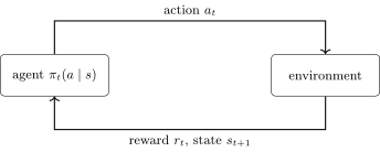
TikZ diagram — The agent's game with the environment: the agent chooses an action by its strategy, the environment responds with a reward and passes into a new state, which it tells the agent.

Our strategy is now not simply a discrete distribution but a conditional discrete distribution. Whereas before $π (a)$ was a normalised non-negative vector, here we have a matrix of size $∣ A ∣ \times ∣ S ∣$ , the set of all actions by the set of all states, and our task is to train this matrix. There really is an element of training here: whereas in the simple case of the multi-armed bandit we train one vector, the strategy, here we train a whole matrix, it has many more parameters, and clearly more rounds have to be played too.

Here there is already a certain theory, based on Markov decision processes. This is a simplifying assumption saying that the probability of seeing such a reward and such a next state, that is, the probability that the environment will pass into a new state and give us a reward, depends not on the whole prehistory but only on the previous state and our action. It does not depend on what was a step back, two steps back and so on: this whole tail plays no role. The Markov property is an important property that very often really holds in practice and is not too burdensome a restriction.

How this differs from ordinary machine learning problems

Remark (How this differs from ordinary machine learning problems).

The sample $(s_{t}, a_{t}, r_{t})$ is not independent.
The distribution $p (s_{t}, a_{t}, r_{t})$ may change over time and depend on the agent's strategy $π$ .
The rewards may be:
- delayed (evaluating actions with a delay);
- sparse (almost all the time $r_{t} = 0$ );
- noisy (it is unclear what exactly the reward is for).

What parametric models can be trained:

the function of the value of an action in a state, $Q (s, a; θ)$ ;
the function of the value of a state, $V (s; θ)$ ;
the strategy $π_{t + 1} (a ∣ s; θ)$ ;
a model of the environment $(r_{t}, s_{t + 1}) = μ (s_{t}, a_{t}; θ)$ .

Let us discuss a little how this formulation differs from ordinary machine learning problems. There is a sample: a sequence of "state, action, reward" triples. But this sample is by no means independent, and most machine learning methods cannot be applied here the way we usually applied them: we need to change the strategy, adjusting it to the changing properties of the environment.

What difficulties are there with the environment itself, which may behave in a non-trivial way? For example, the rewards may evaluate actions with a very large delay. Imagine some computer game: you have a strategy for getting through a level, you take some actions and understand that in five minutes you will reach the end of the level, having collected a heap of goodies and done some non-trivial actions. You will get the reward only in five minutes, when you reach the finale of the level. It is also said that rewards may be sparse: you are playing the game, performing some actions, preparing yourself for the finale that you will reach with the maximal payoff, but so far these actions tell you nothing about what the reward at the end will be. The reward is heavily deferred; it comes not for each of your actions but some time later, and you have to be very far-sighted. It may also be that most of your actions end with a zero reward at the given step, but later it will be returned to you in a large amount. And the rewards may be noisy: the final reward may, generally speaking, depend not only on your actions but also on some random changes in the environment.

These are the conditions in which one has to act. But they are conditions as close as possible to real life: it seems that this is how it is in real life, and so learning in such conditions is a very important skill. It seems that this is a much more adequate model of learning than learning from a sample, as we did before throughout the whole course.

And one more important question: what is it that we are actually training? In the multi-armed bandit we train one vector, the strategy, a discrete distribution. Now that states have appeared, we will have to train a set of such vectors, that is, a matrix. But in general one can introduce parametric models, and today we will see how this is done. Parameters can be introduced into the strategy; into the function that estimates the value of the current state, how profitable it is for you to pass into this state; into the function of the value of an action in a state; we will define what $Q$ and $V$ are in a moment. And finally, the coolest models are those that model the environment directly: a function that returns the reward and the next state, that is, shows how they are functionally connected with the previous state and our action. One can try to build such models, regression ones as a rule, and in them too the parameters have to be trained. As you see, the game is not very simple, and parametric models can be introduced here in as many as four completely different places and trained.

Return and the value of an action

Let us introduce several very important definitions, which in fact make up the ABC of reinforcement learning.

Definition (Return and value functions). The total return on a finite horizon $T$ :

R_{t} = r_{t} + r_{t + 1} + \dots + r_{t + T} .

The discounted return:

R_{t} = r_{t} + γ r_{t + 1} + \dots + γ^{k} r_{t + k} + \dots,

where $γ \in [0, 1)$ is the discount factor; $1 + γ + γ^{2} + \dots = \frac{1}{1 - γ}$ is the agent's horizon of foresight.

The state value function $V^{π} (s)$ and the function of the value of an action in a state $Q^{π} (s, a)$ , given that the agent follows the strategy $π$ :

V^{π} (s) = E_{π} (R_{t} ∣ s_{t} = s) = E_{π} (k = 0 \sum \infty γ^{k} r_{t + k} s_{t} = s),

Q^{π} (s, a) = E_{π} (R_{t} ∣ s_{t} = s, a_{t} = a) = E_{π} (k = 0 \sum \infty γ^{k} r_{t + k} s_{t} = s, a_{t} = a) .

The total return on a finite time horizon. We are at the current moment of time $t$ and have received a certain reward, but our action at this moment may affect future rewards; recall the properties of delay and sparsity. We need to be able to estimate the future total return on some time horizon. But clearly, if we increase the horizon, this sum will accumulate and grow to infinity. So the so-called discounted return is used: the rewards are multiplied by a decreasing geometric progression. $γ$ is called the discount factor; it is less than one, and so the sum of such an infinite series has a finite value. This cannot be said of the total return: it may grow without bound, while the discounted return is already bounded above, if the rewards are bounded, and they are always bounded by some known range for us. The quantity $1/ (1 - γ)$ is called the agent's horizon of foresight. If $γ$ is close to one, this horizon can be quite large; it is, as it were, the effective horizon on which we try to foresee our return.

And the two most important definitions: what the value of a state is and what the value of an action in a state is. The important symbol here is $E_{π}$ : it is the expectation of the discounted return given that we use a fixed strategy $π$ . Let me remind you that a strategy is a family of conditional distributions, in effect a matrix. We consider our strategy $π$ fixed and can find the expectation of the discounted return. The value of an action in a state is a similar thing, only the expectation is taken conditional not only on the state of the environment but also on our action.

What are these value functions needed for? If we have the function of the value of an action in a state, we can of course use it to build very simple greedy strategies: let us take the action that maximises this function. We will little by little justify this strategy now. The stretch here, of course, is that these quantities are defined as expectations under a fixed strategy, while we are playing a game in which we change the strategy at each step. But without such an assumption it will be impossible to build any theory.

The Bellman equation

Let us advance a little in the analytical estimation and derive a very important recurrent formula for the function of the value of an action in a state.

Theorem (Bellman). The recurrent formula for the value function $Q^{π} (s, a)$ :

Q^{π} (s, a) = E_{π} (k = 0 \sum \infty γ^{k} r_{t + k} s_{t} = s, a_{t} = a) = E_{π} (r_{t} + γ k = 0 \sum \infty γ^{k} r_{t + k + 1} s_{t} = s, a_{t} = a) = E_{π} (r_{t} + γ Q^{π} (s_{t + 1}, a_{t + 1}) s_{t} = s, a_{t} = a) .

The Bellman equation for the optimal value function $Q^{*}$ :

Q^{*} (s, a) = E (r_{t} + γ a^{'} \in A max Q^{*} (s_{t + 1}, a^{'}) s_{t} = s, a_{t} = a) .

Proposition. The greedy strategy "choose the action on which the maximum in the Bellman equations is attained" is optimal:

π_{t + 1} (a) = \frac{1}{∣ A _{t} ∣} [a \in A_{t}], A_{t} = Arg a \in A max Q^{*} (s_{t}, a) .

Let us take the infinite sum and detach the first term: for $k = 0$ the first term is $r_{t}$ , and all the other terms are multiplied by $γ$ , so $γ$ can be taken outside the sum. What remains? Still an infinite sum, very similar in appearance to the original one, only it begins at the next moment of time. So, bringing the expectation sign inside, we can replace it by $Q^{π} (s_{t + 1}, a_{t + 1})$ . What have we obtained? A recurrent relation, or more precisely, a huge number of recurrent relations for the elements of this $∣ S ∣ \times ∣ A ∣$ matrix $Q^{π}$ : we have, as it were, expressed it through itself, expressed some "state, action" pairs through other pairs.

And there is the remarkable Bellman equation, which states: if here, under the expectation sign, we put the maximum over all actions, as it were apply the greedy strategy inside this formula, we get a system of equations that defines the optimal value function $Q^{*}$ ; let us call it the Bellman value function. There is a theorem proving that it really is optimal, and this is a certain justification that we may use the greedy strategy if we have learned to estimate $Q$ in this way. The statement is this: the greedy strategy with respect to the optimal value function determined from this system of equations on the matrix $Q (s, a)$ , that is, choosing the action on which the maximum in the Bellman equations is attained, is optimal. This is a theorem; its proof can be found in the book by Sutton and Barto; today we have no time to go into the proof.

So far it is completely unclear to us how to do this: it seems that these relations are very non-constructive, if only because we cannot obtain the expectation. We will now deal with this little by little.

The SARSA method

Let us try to cope with the fact that we do not yet understand how to compute this $E_{π}$ . As always when we compute some expectation, we can estimate it from a sample, approximately, of course. What must we do to estimate this expectation approximately? Compute sums over the prehistory of our whole process of playing with the environment. Here, of course, the exponential moving average comes to the rescue: we can estimate the function of the value of an action in a state approximately as the exponential moving average of the expression that stands under the expectation sign. Running ahead: with the next move we will also put the maximum over all actions here. But for now let us look at a fairly well-known method, SARSA, from the first letters: state, action, reward, state, action.

Definition (The SARSA method). Being in the state $s_{t}$ and having performed the action $a_{t}$ , the agent receives the reward $r_{t}$ and the new state $s_{t + 1}$ , draws the next action by its strategy, $a^{'} \sim π_{t} (a ∣ s_{t + 1})$ , and updates the estimate:

Q (s_{t}, a_{t}) := EMA_{α} (r_{t} + γ Q (s_{t + 1}, a^{'})) = α (r_{t} + γ Q (s_{t + 1}, a^{'})) + (1 - α) Q (s_{t}, a_{t}) .

An on-policy method: the very strategy we are training is used to estimate $Q$ .

What does this mean? Being in some state and having performed an action, we receive a reward, the environment tells us its next state, and at this moment we may not perform our next action but simply draw it: not report the results of the draw to the environment itself, but simply use the result of this sampling. After all, we are building a strategy and are free to see what next action could be drawn if we used it. And at this step the agent, first, uses the greedy strategy, second, draws the next action by its own strategy, and a step of the exponential moving average is made. Such methods are called on-policy algorithms, because the very strategy we are training is used to estimate the function $Q$ . We have updated the value of $Q$ by the exponential moving average for the state $s_{t}$ and the action $a_{t}$ , having looked at what the next state $s_{t + 1}$ and our possible action $a^{'}$ , drawn from our strategy, will be.

Such is the clever trick. Once more: how do we avoid computing expectations over the strategy here? We take the next step, get into the next state and, knowing the next action, can update the estimate $Q (s, a)$ for the previous state and action. We all the time, as it were, run one step ahead in order to update the estimate of $Q$ for the state one step back, and in this way we keep accumulating in the matrix $Q (s, a)$ information about the values of actions in states.

The Q-learning method

Now we take the next step and replace the greedy strategy here by the maximum. This is probably the best-known method; it is called Q-learning: it really approximates Bellman's optimal strategy by means of the exponential moving average.

Definition (The Q-learning method). We approximate $Q^{*} (s, a)$ by the exponential moving average:

Q (s_{t}, a_{t}) = EMA_{α} (r_{t} + γ a max Q (s_{t + 1}, a)) .

Initialisation of the strategy $π_{1} (a ∣ s)$ and of the state of the environment $s_{1}$ ;
for all rounds $t = 1, \dots, T, \dots$ :
- the agent chooses an action $a_{t} \sim π_{t} (a ∣ s_{t})$ ;
- the environment generates $r_{t} \sim p (r ∣ a_{t}, s_{t})$ and $s_{t + 1} \sim p (s ∣ a_{t}, s_{t})$ ;
- $Q (s_{t}, a_{t}) := α (r_{t} + γ max_{a} Q (s_{t + 1}, a)) + (1 - α) Q (s_{t}, a_{t})$ .

Proposition. If $α_{t}$ decreases ( $\sum_{t} α_{t} = \infty$ , $\sum_{t} α_{t}^{2} < \infty$ ) and all pairs $(s, a)$ are visited an infinite number of times, then $Q \to Q^{*}$ almost surely as $t \to \infty$ .

An off-policy method: the strategy for choosing actions $π_{t} (a ∣ s_{t})$ may differ from the greedy strategy $a_{t} \in Arg max_{a} Q (s_{t}, a)$ that we are estimating, for example be ε-greedy on the basis of $Q$ .

Here we average by the exponential moving average exactly the quantity that stands in the Bellman equation, and as before we use the information about the future state to update $Q$ for the previous state. Such strategies are called off-policy. Why is this important? Here we get a certain freedom in using the strategy. The strategy $π$ may be Bellman-optimal, but not necessarily: for example, we can mix it with an ε-greedy strategy, with a uniform distribution, modify it in some other way. Such algorithms are called off-policy because the strategy for choosing actions may differ from the one we are trying to estimate, and that one will be close to the optimal, Bellman one.

A whole heap of different theoretical statements have been proved about such games. In particular, one of them: if we decrease $α_{t}$ over time, but neither too fast nor too slowly, and if we guarantee that all states are in the end visited an infinite number of times, then such a function $Q$ will converge to the optimal Bellman function as the game tends to infinity. That is, it was not for nothing that we put this construction here: it really is close to the optimal one and tends to it asymptotically.

If you have not understood what Q-learning is, it will be rather hard from here on: we are now going to make things more complicated.

Deep Q-learning: Atari games

Q-parametrisation on the example of learning Atari games

Let us go further, into cool things: Atari games. This is a much-publicised result published in 2013 by the DeepMind team. They showed that in an environment of computer games, simple arcade games that ran on the old Atari computers, reinforcement learning techniques can train a model that will itself learn to play this game and to win. We put in neither the rules of the game nor our assumptions about the strategy; we put in only the set of possible actions. The system sees only what the player sees on the screen, the frames of the game, and the score.

Definition (Q-parametrisation on the example of learning Atari games).

The environment is an emulator of 7 Atari games, each frame $210 \times 160$ pixels, 128 colours.
The states $s$ are 4 consecutive frames, compressed to $84 \times 84$ .
The actions $a$ : from 4 to 18, depending on the game.
The rewards $r$ : the current SCORE according to the rules of the game.
The value function $Q (s, a; w)$ is a CNN with input $s$ and $∣ A ∣$ outputs.

V. Mnih et al. (DeepMind). Playing Atari with deep reinforcement learning. 2013.

First, they built a simulator of the Atari computer; seven games run on this simulator. Each frame is $210 \times 160$ pixels, 128 colours; such are the properties of this emulator. Then we have to agree on how our game is arranged: what a state is and what an action is.

States we will call four consecutive frames of the game. Why exactly four? They probably tried different numbers. If we take fewer, we do not have enough information about how the action is unfolding at the moment, who is flying in which direction; for that at least four frames are needed. And if there are more frames, it is apparently practically useless and only loads the model. Exactly four frames were chosen from some such considerations. Then these frames are for some reason compressed to the size $84 \times 84$ . One would think they need not be compressed; well, they gained roughly six times in memory. How worthwhile that gain is, and whether ten years later this model could not be redone so as not to have to sacrifice pixels, I do not know. That is how they did it then; probably something did not fit into memory.

Next, the most interesting thing: the actions. Each game has its own set of buttons that the user presses: from 4 to 18 actions in different games. And we want to build a universal architecture that observes these pictures: the state $s$ is four consecutive pictures, and we already see that we will need convolutional neural networks for processing images. We do not even want to tune to the game: we want one universal architecture to play all seven games, regardless of the number of actions in the game and of the meaning of these actions. For us the actions are initially equal in rights, equally probable: we do not understand which of them is more profitable and which more important for the game.

The reward is the current score, computed according to the rules of the game. Here, of course, we do not peek at how this score looks in the frame: such a problem is not being solved, thank God. Since we have an emulator, we know the current score inside it and can take it directly from there.

And then the most interesting thing: how the value function is modelled. Here for the first time we encounter a parametric model of the function of the value of an action $a$ in a state $s$ being introduced, and not only a parametric one, but a deep neural network at that. At the input is the state, four consecutive frames of this size; then two convolutional layers, in which the size decreases and the dimension grows, and at the end we get a vector of 256 mysterious coordinates, some embedding of this state. That is, we have translated the state, four consecutive frames, into a vector of dimension 256 and hope that it will contain complete information about which actions are more profitable and which less. Then one more fully connected layer, which at the output gives us the estimates of the actions, that is, a vector of dimension $∣ A ∣$ .

Why did they do it exactly like this, rather than feed the state and the action to the input explicitly? After all, the function $Q$ takes a state and an action as input. Probably it could have been done that way too, but the authors preferred the path where the state is given at the input and at the output we get the estimates of all actions; mathematically these are equivalent things. The main thing is that these are two convolutional layers followed by two fully connected ones. Not such a deep network, and not such a huge number of parameters. Nevertheless this contraption turned out to be quite successful in solving these problems.

To the point that, for example, in Breakout, a game in which we control a paddle at the bottom and a ball flies about, there is an optimal strategy: you have to knock a hole through to the ceiling and send the ball there, and then the ball starts flying between the top layer and the ceiling and knocking out all the bricks. This is a winning strategy. And on the example of this game it was shown that, although nobody taught the algorithm to apply precisely this strategy, the algorithm itself discovered that this trick works and began to use it. This example is always given to astonish people with how great the learning abilities of this approach are.

The DQN method

Let us look into the features of this method: how the deep neural network is actually trained. It is called the Deep Q-Learning Network: it is the very Q-learning we have already seen, but here there is also a neural network that has to be trained.

Definition (The DQN method (Deep Q-Learning Network)). Storing the trajectories $(s_{t}, a_{t}, r_{t})_{t = 1}^{T}$ in memory (replay memory) for repeated reproduction of experience (experience replay).

Approximating the optimal value function $Q (s_{t}, a_{t})$ with the current network parameters $w_{t}$ fixed:

y_{t} = {r_{t}, r_{t} + γ max_{a} Q (s_{t + 1}, a; w_{t}), if the state s_{t + 1} is terminal, otherwise .

The loss function for training the neural network model $Q (s, a; w)$ :

L_{t} (w) = (Q (s_{t}, a_{t}; w) - y_{t})^{2} .

Stochastic gradient SGD (by mini-batches of length 32):

w_{t + 1} = w_{t} - η (Q (s_{t}, a_{t}; w_{t}) - y_{t}) \nabla_{w} Q (s_{t}, a_{t}; w_{t}) .

V. Mnih et al. (DeepMind). Playing Atari with deep reinforcement learning. 2013.

There is one more interesting feature: trajectories are stored in memory, replay memory: a certain prehistory of the game is kept in memory all the time so that we can reproduce it many times. This is called experience replay, and on these pieces of the game our neural network is trained by the stochastic gradient method.

Next we build an approximation of the optimal value function with the current network parameters fixed. What do we train on? We will train a regression model $Q$ : it must predict $y_{t}$ . $y_{t}$ is arranged like this: it is either the final reward, if we have come to a terminal state, the game is over, we have got the score, and the larger it is, the better; or, if we are not in a terminal state, our usual expression that we average. That is, when we do stochastic gradient by mini-batches, we will in effect be training on $y_{t}$ , exactly as in Bellman's optimality equations.

The loss function itself for training the neural network model is as in the method of least squares; this is for one round of the game, but we will train by mini-batches. What is a mini-batch? It is short fragments of 32 rounds, that is, 32 states; I draw your attention to the fact that each state is also four consecutive frames, so 32 states is a fairly large stretch of the game. Training on such a mini-batch, we perform stochastic gradient descent and tune the parameters $w$ . Here is the formula for how $w$ changes; the most important thing here is to compute the partial derivatives, but that is done, as usual for deep neural networks, by ordinary backpropagation; there is nothing special here. The main thing is how to connect backpropagation for a deep neural network with Q-learning, and that is exactly what is shown on this slide.

DQN: putting it all together

Definition (The DQN method: the algorithm).

Initialisation of the replay memory and of the network parameters $w$ ;
for all episodes $m = 1, \dots, M$ :
- initialisation of the state of the environment $s_{1}$ ;
- for all $t = 1, \dots, T_{m}$ (the length of the $m$ -th episode):
  - $a_{t} = {a random action, ar g max_{a} Q (s_{t}, a; w), with probability ε, with probability 1 - ε;$
  - the environment generates $r_{t} \sim p (r ∣ a_{t}, s_{t})$ and $s_{t + 1} \sim p (s ∣ a_{t}, s_{t})$ ;
  - store $(s_{t}, a_{t}, r_{t})$ in the replay memory;
  - choose a random fragment of a trajectory from the memory;
  - for all $j = 1, \dots, J$ (the length of the mini-batch): estimate $y_{j}$ ; take a gradient step, update $w$ .

V. Mnih et al. (DeepMind). Playing Atari with deep reinforcement learning. 2013.

Let us put everything together, to understand once more how it works. We first initialise the memory, initialise the network parameters and begin going through episodes of the game, $t$ from one to $T_{m}$ , the length of the episode; clearly, games may be of different lengths. We play with the Atari emulator. At the moment of time $t$ , with some probability, we take random actions: we need the exploration–exploitation trade-off, after all; we have first to play a little, simply performing different actions at random and observing what results this leads to. Or we already operate by the greedy, Bellman strategy with the value function we have estimated by this moment.

Then the environment, in response to our action, generates a reward and passes into a new state: the frame has changed. We store the "state, action, reward" triple in a certain buffer in memory. We cannot store the whole prehistory of the game, simply because no memory would be enough; this buffer is of quite limited size, and the latest fragment keeps displacing an older one. Then we choose a random fragment of a trajectory from among those stored in memory and take gradient steps on the mini-batch. That is really all.

This is DeepMind's brilliant 2013 paper; it made a great stir, and there was a great deal of hype of every kind about it: to this day people write that artificial intelligence learned by itself, by reinforcement learning methods, to play Atari games, even without any hints from people. Previous work was about people sitting down, playing the game, and the algorithm learning from the video. Here the algorithm simply plays with the Atari emulator and achieves by itself an understanding of how the game should be played: having played a huge number of rounds, it understands what actions have to be performed in the current state. Such is the interesting paradigm. I tried to tell this very interesting story very concisely, in three slides; if it interests you, read the original paper. But it is already considered outdated, 2013 after all: a great deal has been done since, and these reinforcement learning strategies have been taught to play many different games.

Remark (Watching a human or playing oneself). What is the conceptual difference between the situation where we watch a human play and draw conclusions from it, and the situation where we first poke around at random ourselves? When a human plays, we follow the teacher's actions and consider that this is a good player, but we can learn only his strategy: if the teacher does not show something, we are unlikely to make a discovery ourselves. And when the artificial intelligence itself chooses the actions in the game, at first, of course, there will be some absurd attempts to perform wrong actions, but the learning happens quite fast: the computer plays with itself, there are no delays connected with human reaction, and all this can be played through insanely fast. Playing on its own, the strategy can learn techniques that, for example, a human does not know, and this is a way of making new discoveries in how one should interact with the environment. So playing on one's own is a more advanced way of learning than watching how a human teacher plays.

In terms of the functional principle, in both cases we look at the state, at the action and at what comes of it. But the main difference is that in the recording of a human's game we know only the actions he performed, and nothing can be changed in the fixed recording of the teacher's actions. Here, by contrast, we can try any actions ourselves: if the situation occurs again, we can play differently. In a recording we cannot experiment actively; that is the main difference.

Gradient optimisation of the policy

Policy gradient

I draw your attention to what we trained here: we trained the value function of an action in a state. We understand that the state space here is so huge, four consecutive frames, anything at all can be there, that we will of course be unable to accumulate the responses for each such state and estimate $Q (s, a)$ adequately as if it were simply a "state by action" matrix. That cannot be done, so a parametric model is introduced there, and we build this parametric model as a convolutional neural network. That is one paradigm.

A completely different paradigm is when we introduce the parameters into the agent's strategy. This is another case, and here one of the best-known training methods is called policy gradient.

Definition (Gradient optimisation of the policy (policy gradient)).

$π (a ∣ s, θ)$ is the agent's strategy with parameter $θ$ ;
$F (s_{t}, a_{t})$ is the value function or an estimate of it (for example, $R_{t}$ ).

The problem of maximising $E_{π} F$ over the vector of strategy parameters $θ$ :

E_{π} F (s, a) \equiv E_{a \sim π (a ∣ s, θ)} F (s, a) \to θ max .

The gradient method: $θ^{(t + 1)} := θ^{(t)} + η \nabla_{θ} E_{a \sim π} F (s, a)$ , where

\nabla_{θ} E_{a \sim π} F (s, a) = \nabla_{θ} a \in A \sum F (s, a) π (a ∣ s, θ) = a \in A \sum F (s, a) \nabla_{θ} π (a ∣ s, θ) = a \in A \sum F (s, a) π (a ∣ s, θ) \frac{\nabla _{θ} π ( a ∣ s , θ )}{π ( a ∣ s , θ )} = E_{a \sim π} (F (s, a) \nabla_{θ} ln π (a ∣ s, θ)) .

R. Sutton et al. Policy gradient methods for reinforcement learning with function approximation. NIPS 1999.

Suppose we are going to measure value somehow. It may be $Q$ , it may be $V$ , it may be simply the discounted returns $R_{t}$ themselves: value can be measured in different ways. For generality let us say that it is simply some function $F$ of an action in a state that we can compute. Why introduce such a parametrisation? For the same reason as in the previous case: the set of states may be so rich that we simply cannot accumulate the strategy as an "action by state" matrix. So we introduce a parametrisation, and the problem is to maximise the expectation of the value function over the strategy.

And here arises the greatest non-triviality, which at first sight is baffling, because we have not seen anything like it until now. We need to maximise the expectation of the value function, while the parameters $θ$ that we are going to train sit not in the loss function, as usual, but in the distribution from which we are going to sample actions and then estimate the expectation over all possible variants. At first sight it is just some kind of horror: the parameter $θ$ sits in the expectation, and what is to be done with that? Yet we want to train this parameter.

But if we carefully write out what the expectation is and how we will look for the gradient with respect to the parameter $θ$ , we will see that there is nothing complicated here. Let us write out the expectation: it is the sum over all actions of $F$ multiplied by the probability of the given action, which has the parameter $θ$ . This is already a perfectly clear formula for us, containing a function $π$ that is, we hope, differentiable. Let us bring the gradient under the summation sign: $F$ does not depend on $θ$ . Now let us do this trick: divide and multiply by $π (a ∣ s, θ)$ . The ratio of the gradient of $π$ to $π$ itself is the gradient of the logarithm of $π$ , and what is left is again the formula of an expectation over actions from our parametrised strategy.

What is the bonus? Now the gradient with respect to the parameter $θ$ applies to an explicitly written function: it has been brought inside the expectation. We no longer need to differentiate with respect to the parameters of the distribution over which the expectation is taken: we have brought the differentiation with respect to the parameter inside the expectation. And a remarkable thing has come out: we will have to differentiate the logarithm of the probability of actions as a function of the parameter $θ$ . What does this resemble? The maximum likelihood principle, of course. One has the feeling that the value function plays the role of the empirical distribution, and under the logarithm is the model distribution. That is, this can be interpreted as the maximum likelihood principle, or at least something very similar to it, or as cross-entropy. This is already our old acquaintance, and we know how to solve such problems.

The connection with log-likelihood maximisation

Definition (Policy gradient as log-likelihood maximisation). Replacing $E_{π}$ by an empirical EMA estimate of the gradient:

θ^{(t + 1)} := θ^{(t)} + η EMA_{α} (F (s_{t}, a_{t}) \nabla_{θ} ln π (a_{t} ∣ s_{t}, θ^{(t)})) .

In effect this is stochastic gradient SGD with B. T. Polyak's momentum method for maximising the log-likelihood:

t \sum F (s_{t}, a_{t}) ln π (a_{t} ∣ s_{t}, θ) \to θ max .

The main differences from log-likelihood maximisation:

instead of predicting class labels $y_{t}$ , the actions $a_{t}$ ;
instead of binary $y_{t}$ , real-valued $F (s_{t}, a_{t})$ .

What can be used as $F (s_{t}, a_{t})$ :

the return function $R_{t}$ ;
the value function $Q (s_{t}, a_{t})$ ;
the advantage function $Q (s_{t}, a_{t}) - V (s_{t})$ .

So we have replaced the expectation over the parametrised strategy by an empirical estimate as well, an exponential moving average, and then we have got altogether the familiar stochastic gradient method, in which we also know how to average the gradient by an exponential moving average in order to move faster in the direction of the steepest descent of the criterion. Recall the method of moments, momentum, Polyak's heavy-ball method. That is, this is simply the very stochastic gradient method for maximising a functional that can already be considered a log-likelihood: here is the probabilistic model, and the value function in effect plays the role of the empirical distribution; these are our empirical data.

The main difference from log-likelihood maximisation in classification problems is that usually we predict class labels, while here actions are predicted. But both are finite sets, that is, a complete analogy with how we solve classification problems: we have here a decision-making problem on a finite set; in essence this too is classification. And instead of training on some binary answers of a teacher, here it is a little trickier: we train on a real-valued value function $F$ , whatever it may be.

And what can it be? Once more: it can be the return $R$ , the function of the value of an action in a state, the state value function $V (s)$ , but that is not often done. People also take an estimate of the advantage: we saw such a quantity once today, at the beginning. It is the function of the value of an action in a state compared with the state value function, which is, as it were, averaged over all actions. That is, we have already introduced the quantities $Q$ and $V$ . In principle, different things can be taken as $F$ , and sometimes one works better, sometimes another; people simply experiment with what is better to maximise in a particular problem.

Once more: policy gradient is an approach to parametrising the agent's strategy. Remember, we talked about what can be trained at all in such problems, and there are many options. We have now considered how to train the strategy; on the example of Atari games we saw how to train the value function of an action; the value of a state we will not go into, it is roughly analogous there. And now it is time to move on to how the parameters of a model of the environment can be estimated, and this is of course the most non-trivial, the most interesting, the most advanced case.

Modelling the environment

Model-based and model-free

One more topic remains: how to model the environment. Here there is a major division of reinforcement learning methods into model-based and model-free. In my view this is not a very fortunate formulation: when we introduce some parametric model, and we have just looked at two such variants, that is a model too. Nevertheless all this is called model-free, because model-based reinforcement learning is customarily understood to mean precisely modelling the environment.

Definition (Modelling the environment in reinforcement learning). How model-based approaches differ from model-free ones:

the behaviour of the environment $(r_{t}, s_{t + 1}) = μ (s_{t}, a_{t}; w)$ is modelled;
long-term planning of actions is possible;
a continuous parametrisation of both $A$ and $S$ is possible;
in simple technical control systems an adequate parametric model of the environment may be known.

The difficulty of the problem:

complex environments require large samples to train high-dimensional models;
RL may function well in a simulated environment and much worse in the real one.

T. Moerland, J. Broekens, C. Jonker. Model-based reinforcement learning: a survey. 2020.

A predictive model is built: from the current state and the action in this state it literally predicts what the reward and the next state given by the environment will be. Observing how the environment reacts to our actions, we want to model the law of its behaviour. We are literally doing the work of a natural scientist: we want to find out the law by which this environment functions. This is probably the hardest thing one can try to do here, and the coolest approach.

Why is this important? If we have cracked the environment, understood by what laws it functions, we can do long-term planning of our actions. We can play with this environment as if playing many moves ahead, because we know how it will respond to our actions, if, of course, we have built the model well. Such anticipatory interaction with the environment is in the long run the most profitable way to beat the environment. This is often used in controlling technical systems: even if the system is very complex, we can still try to model it somehow. For complex technical systems, for robots, for industrial production, approaches of this sort are often used, because we know a great deal about the environment: we ourselves constructed this environment as a certain physical object. Even in this case it is not always possible to build ideal models, but one can model quite well.

The difficulties of this problem are that complex environments require very large samples, and also that the model may turn out to be inadequate: in the simulated environment we will function well, and when we move to the real environment, everything there will be much worse. This danger too exists in principle.

Regression with incremental learning and a confidence bound

Let us look at a special case where we model only the reward function for an action and do not model the function of transition to the next state. This is a somewhat cut-down formulation of the problem, but it is still model-based, a simplified variant; for the complex variants we have neither the time nor the strength today. Let us see how incremental regression can be used to solve such problems.

Definition (Regression with incremental learning and a confidence bound).

$r^(s, a; w)$ is a regression model of the reward with parameter $w$ ;
$UCB (s, a)$ is an upper bound of the deviation $r^- r$ ;
$δ$ is a parameter (the larger it is, the more exploration);
the strategy is to maximise the estimate of the reward for $a_{t}$ in $s_{t}$ .

The agent's game with the environment: initialisation of the parameters $w$ of the reward model; for all rounds $t = 1, \dots, T, \dots$ :

the agent chooses the action $a_{t} = ar g a \in A max (r^(s_{t}, a; w) + δ UCB (s_{t}, a))$ ;
the environment generates $r_{t} \sim p (r ∣ a_{t}, s_{t})$ and $s_{t + 1} \sim p (s ∣ a_{t}, s_{t})$ ;
the regression $r^(s, a; w)$ is further trained on the point $(s_{t}, a_{t}, r_{t})$ .

Lihong Li, Wei Chu, John Langford, Robert E. Schapire. A contextual-bandit approach to personalized news article recommendation. WWW-2010.

We have a function of the reward for an action in a state. We do not know this function, the environment knows it, but we try to make a regression estimate of it, and for this we use a parametric model. Parametric models can, naturally, be different, neural networks can be used, but now we will try a simpler variant, a linear model. What else will we need? Recall the upper confidence bound: now we will need upper confidence bounds specifically for linear regression.

What does the agent's game with the environment look like, how does it differ from the usual one? We will use a greedy strategy, but not entirely greedy. We will use a regression estimate of the reward function, tune this function to the real rewards we receive from the environment, and slightly relax the greedy strategy by the upper bound. It gives us the possibility of performing exploratory actions, using a well-founded probabilistic estimate, the upper confidence bound: less explored actions more often get the maximal value, so that they are chosen more often. As soon as we explore an action more, the upper confidence bound decreases, and accordingly we choose this action less often if it is not very profitable. Such is the balance between using the estimate of the rewards and the upper bound.

And the main feature of the model-based approach is that now at each step we need to further train the regression on the point just obtained. In the state of the environment $s_{t}$ we performed the action $a_{t}$ and received the reward $r_{t}$ for it: the "action, state" pair is our object for the regression, and the target quantity is the reward $r_{t}$ . We keep further training the regression on the point we get in the current round. Recall the last lecture: incremental algorithms are of course very much in place here. In general, reinforcement learning is incremental by its nature, and all the models we build there we will keep training incrementally. While we were talking about convolutional neural networks, everything was clear with incrementality: it is stochastic gradient; but here we will have to use incremental methods of linear regression specifically.

An example: recommending news articles to users

A real case, a fairly old one, but nevertheless an example of such a model-based approach and of a perfectly live applied problem: recommending news articles to the users of a news service. A user sees a certain news item, reads it, and the task of the recommender system is to show good recommendations in four positions below, so that the user clicks with high probability on one of the news items offered.

Example (Recommending news articles to users).

The agent is a recommender system for personalising the display of news articles (Yahoo! Today); F1…F4 are the positions for showing news headlines.
$A$ are the news articles, the system's actions.
$s_{t}$ is the state = the user to whom we give a recommendation.
$x_{t a} \in R^{n}$ is the feature description of the pair $(s_{t}, a)$ .
$r_{t a} \in {0, 1}$ is the reward = [the user $s_{t}$ clicked on the article $a$ ].
$Q_{t} (a)$ is the mean reward, the CTR (click-through rate) of the article.
The goal is to raise the mean CTR and "the user's happiness".

Lihong Li, Wei Chu, John Langford, Robert E. Schapire. A contextual-bandit approach to personalized news article recommendation. WWW-2010.

Let us figure out what is the agent, what is the state, what is the action. The agent is the recommender system. What is the set of actions? At first sight it seems that the actions are the four positions; in fact nothing of the kind. The actions are all the news articles that the system is ready to show at the given moment of time: recent news, today's news, for example, that is, of the order of several thousand news articles. One could consider finer actions, in which of the four positions to put a news item, and then this would have to be multiplied by four as well. But here we do not do that: we consider that the four chosen news items are somehow prioritised by a separate algorithm and laid out over the four slots. That is a problem of another kind, and we do not consider it.

Now, what is a state from the point of view of our agent, the recommender system? The state is our user: he has come, is reading this news item, and we know something about him: his previous interests, what news he has already read on our site before, perhaps something else. We must characterise this state by a certain feature description; a little later I will say what the user's features may be. $x_{t a}$ is the feature description of the pair: the state $s_{t}$ is the user, and we need some information about him, about his interests; $a$ is a news article. The features must characterise how well the information in the article $a$ suits the user's interests, that is, the state $s_{t}$ .

Next, how the rewards are arranged in this problem, what success is for our agent. Success is when the user has clicked on one of these four banners. Let us measure the mean reward as is customary both in advertising networks and in search engines: there is a quantity there called the click-through rate, CTR. One can say it is the frequency estimate of the probability that the user will click on the given banner, in this case on one of the four. If the user clicked, the reward equals one; if not, zero. Our task is to collect information about clicks and maximise the probability of a click, that is, the goal is to raise the mean CTR. We consider that it characterises the user's happiness: the user is happy with our system if we often offer him something he clicks on with pleasure.

The linear reward model and LinUCB

Let us see how this problem is solved. Here there is linear regression; $x_{t a}$ are the feature descriptions of our actions in states, that is, of how the article $a$ matches the user $s_{t}$ who came at the moment of time $t$ .

Definition (The linear reward model and ridge regression). Let $x_{t a} \in R^{n}$ , $w_{a} \in R^{n}$ .

The linear reward model for the action $a \in A$ in the state $s_{t}$ :

E (r_{t a} ∣ x_{t a}) = ⟨ x_{t a}, w_{a} ⟩ .

Ridge regression: training $w_{a}$ for the action $a$ at the moment $t$ :

i = 1 \sum t [a_{i} = a] (⟨ x_{ia}, w_{a} ⟩ - r_{ia})^{2} + τ ∥ w_{a} ∥^{2} \to w_{a} min,

w_{a} = (F_{a}^{T} F_{a} + τ I_{n})^{- 1} F_{a}^{T} y_{a}

is the solution of the least-squares problem, where

$F_{a} = (x_{ia})_{i = 1, \dots, t : a_{i} = a}$ is the $ℓ \times n$ "objects–features" matrix;
$y_{a} = (r_{ia})_{i = 1, \dots, t : a_{i} = a}$ is the $ℓ \times 1$ vector of answers;
$ℓ = k_{t} (a) = \sum_{i = 1}^{t} [a_{i} = a]$ is the size of the training sample.

I will not go on to describe very tediously and in detail how this model is built: it is clear that there are feature descriptions here, and how to formalise the criterion for building the model. In this case ridge regression is used, because the parameter space may be fairly large, and ridge regression is used so that there is no overfitting. One could use elastic net or something else, but the authors of the paper preferred ridge regression.

Next an interesting point: precisely for linear regression there are analytical formulas for upper confidence bounds.

Definition (LinUCB: a linear model with an upper confidence bound). The confidence interval with confidence level $1 - α$ for the linear regression model $w : ∥ F w - y ∥ \to min_{w}$ :

y = ⟨ x, w ⟩ \pm σ^Z_{α} x^{T} (F^{T} F)^{- 1} x,

$Z_{α} \equiv t_{ℓ - n, 1 - \frac{α}{2}}$ is a quantile of Student's distribution;
$σ^^{2} = \frac{1}{ℓ - n} RSS$ is the estimate of the variance of the response $y$ .

The strategy $π_{t} (a, x) = \frac{1}{∣ A _{t} ∣} [a \in A_{t}]$ is the action with the maximal upper value estimate UCB (upper confidence bound):

A_{t} = Arg a \in A max (⟨ x_{t a}, w_{a} ⟩ + δ σ^Z_{α} x_{t a}^{T} (F_{a}^{T} F_{a} + τ I_{n})^{- 1} x_{t a}) .

The larger the parameter $δ$ , the more exploration.

If we solve such a regression problem, here in slightly simplified notation, I do not put the index $a$ on the matrix $F$ and on the vector $w$ so as not to clutter the formula, there is a formula given in any statistics textbook: the confidence interval for the predicted quantity $y$ . $y$ is predicted by a linear model, as usual a scalar product, plus or minus the confidence interval, which is set by the quantile $Z_{α}$ ; a quantile of Student's distribution appears here, but one can consider it just some number. If we decrease $α$ , that is, want to increase the confidence level $1 - α$ , the interval widens, $Z_{α}$ increases. What one has to understand qualitatively about $Z_{α}$ : it is some small number, of the order of two.

This formula says that the interval depends, generally speaking, also on how much multicollinearity there is in our model. That is what ridge regression is introduced for: so that this interval does not come out too large because of multicollinearity. So in the formula for ridge regression here there is also $+ τ I_{n}$ , where $τ$ is the regularisation coefficient. In the end we get this strategy of choosing the action with the maximal upper estimate: a linear regression model that predicts the rewards, plus the upper confidence bound. And $δ$ is a parameter that allows the exploration–exploitation trade-off to be controlled: the larger $δ$ , the more often we will take exploratory actions.

LinUCB: implementation features

Remark (LinUCB: implementation features and generalisations).

An incremental algorithm for recomputing $w_{a}$ and the matrix $(F_{a}^{T} F_{a} + τ I_{n})^{- 1}$ when each row is added to $F_{a}$ .
A hybrid linear model $Q^{*} (a) = ⟨ x ~_{t}, v ⟩ + ⟨ x_{t a}, w_{a} ⟩$ , where $x ~_{t}$ is the part of the context that does not depend on the action $a$ .
"Raw features": users, 12 socio-demographic, 200 geographic, about 1000 categories; articles, about 100 categories.
Clustering and dimensionality reduction are used: $dim w_{a} = 6$ , $dim v = 36$ .
Any other model with incremental learning and confidence bounds could have been used.

A few more features of this model. First, as I have already said, an incremental recomputation algorithm is used. Last time we already looked at how the Sherman–Morrison formula works; now it is used with the ridge added as well.

Next, the feature descriptions: what the features are is of course the most interesting part. We use features that depend either on the article or on the user. User features are socio-demographic characteristics: it turns out the service knows a great deal about the user, including the level of education, age, sex. Then geography, that is, where the user makes requests from, from which state. And information about categories is known: texts are categorised, and the user's interests are categorised too. This can be done in different ways, I will not even go into the details: clearly one can use clustering methods, even topic modelling. In this paper the categorisation was done by clustering. After all these contrivances the dimension is greatly reduced, and these parameters in the model have dimension 6. But note: there are many articles. For each $a$ , and these are our actions, the articles we recommend, there is its own parameter vector of length 6. If today the pool of recommended articles contains, for example, five thousand articles, then 5000 has to be multiplied by 6, which is also quite a lot. And there are features common to all $a$ ; they too make up part of the feature description.

In fact such a model could have been built in many different ways. It was by and large the choice of the authors of this work: why they used exactly this feature description, exactly linear regression, exactly with this regularisation and not some other is of course a matter of taste. But at the same time it is an interesting case that shows the main thing: how one can model the function that predicts the reward and build a model of the environment.

Evaluating the model on historical data

And the last point connected with this case. It is interesting because a similar strategy is very often used in various internet services, search and recommender ones, when recommendations are built with reinforcement learning and they have to be adjusted very quickly to particular users.

Definition (Evaluating the model on historical data). The problem of off-line evaluation of a strategy $π$ : the historical data were accumulated while using another strategy (logging policy) $π_{0} (a)$ , different from $π$ .

The idea: to estimate $Q_{t} (a)$ , only those events $(x_{t a}, a, r_{t a})$ are selected for which the strategies $π$ and $π_{0}$ chose the same action:

a = ar g a max π (a, x_{t a}) = ar g a max π_{0} (a)

(very large data or similarity of the strategies are needed).

Proposition. If $π_{0} (a)$ is the uniform distribution, the estimate of $Q_{t} (a)$ on the selected sample is unbiased.

Lihong Li, Wei Chu, John Langford, Robert E. Schapire. A contextual-bandit approach to personalized news article recommendation. WWW-2010.

The problem of offline evaluation: we want to evaluate a certain new strategy, but we understand that the historical data on which we build our regressions were in their time also formed by some strategy, but a completely different one. This other strategy is called the logging policy, and it of course differs from the strategy we are now trying to optimise. Training on these data is not entirely correct, since they were formed by another strategy. In particular, if the old strategy did not suggest some right article to a user, while our strategy sees that this article should be recommended to this user, we have no way of evaluating the quality of this recommendation on the historical data. Something has to be done about this.

The idea here is very interesting, and it clearly exploits the fact that our amount of data really is gigantic: this is genuine, real big data, and such things can be done with it. To estimate the value function $Q_{t}$ we can select from the historical data only those events on which the answers of our strategies coincided: to use for evaluating our strategy $π$ only those articles that were offered to the user by the old strategy $π_{0}$ , the logging policy that was working at the time our training data were formed. Such is the trick. It is a certain filter that will of course select some small share of the big data, perhaps one per cent, perhaps ten per cent of the data, God knows. The requirement that the recommendations of the two strategies, the logging policy and the one we are now building, coincide may carve a small share out of the sample, but there are so many data that even this share will be statistically representative. It is an interesting technique that may be useful in many other places.

Summary

In reinforcement learning there are no teacher's answers, there is only the response of the environment.
What can be trained in model-free approaches:
- the value function $Q (s, a; w)$ , for example by SGD;
- the strategy $π (a ∣ s; w)$ , by policy gradient;
- the models of the actor $a (s; w_{1})$ and the critic $Q (s, a; w_{2})$ .
What can be trained in model-based approaches:
- only the reward model $r (s, a; w)$ ;
- a model of the environment $(r_{t}, s_{t + 1}) = μ (s_{t}, a_{t}; w)$ .
The exploration–exploitation trade-off in any reinforcement learning is chosen experimentally.

R. S. Sutton, A. G. Barto. Reinforcement Learning: An Introduction. 2018. https://spinningup.openai.com/en/latest Yuxi Li. Resources for Deep Reinforcement Learning. 2018.

I again give references to the book by Sutton and Barto and a couple more useful links: OpenAI has very good documentation on reinforcement learning, and there is one more survey of resources on deep reinforcement learning, with very many interesting links; if anyone is interested in this, I recommend finding it and having a look.

Briefly: today we have considered many different approaches to parametrisation. How to parametrise the strategy: that is policy gradient. How to parametrise the function of the value of an action in a state: that is how learning Atari computer games by interacting with the emulator is arranged. And how model-based models that try to model the environment are arranged; true, today our example came out cut down: we modelled only the rewards and did not model the function of transition to the next state. There is also a remarkable approach called "actor–critic", but we did not get to it at all, and I did not even aim to get round to telling about it. It is the simultaneous modelling of both the action in a state and the function that estimates the value of an action in its state: two such models are built at once, and each has its own parameters that are trained.

And the last thought: the exploration–exploitation trade-off takes place in absolutely all these models, and everywhere one has to introduce some parameter that controls this trade-off and tune it somehow. At the beginning one has to explore more, to perform perhaps more random actions; then, as we learn more about the environment and model it better, we pass from exploration to exploitation more and more often.

Remark (Reinforcement learning or incremental learning). Which do modern search and recommender systems use more, reinforcement learning or simply incremental algorithms? It differs from place to place. If we need to react very quickly to a user's rapidly changed interest, reinforcement learning can really help here. If, on the other hand, we focus on the longer-term interests of users, we can, for example, update the model once a day and use more static models. In general, the dilemma of whether to use classical machine learning or reinforcement learning is connected precisely with whether we have a training sample where the answers have been prepared in advance by a teacher, or an environment with which we interact, as in robotics, in training robots. If a training sample is formed, classical machine learning methods will simply work more efficiently. Reinforcement learning is a more complex approach: the response of the environment is not easy to model, and training usually requires a much longer history, that is, more data. The approach is more capricious, reinforcement learning models are harder to build, and the game must be worth the candle. You must understand that you really have a problem in which you cannot afford to accumulate a training sample and then tune on it, or perhaps cannot afford even plain incremental learning, because you have no teacher's answers but only some response of the environment. And if the response of the environment is, as we said, sparse, delayed and noisy, there are no options other than reinforcement learning. If you need to learn to control a robot, to play a computer game, or in general to interact with a complexly arranged environment and accumulate experience, a training sample will not help you, however incremental the learning: you will not be able to take these features of reinforcement learning into account.

Seminar

Watch on YouTube

Voron-ML-RL-slides.pdf