August 30, 2026 · Lecture · LibreTimes
Machine Learning 2. Lecture 9. Incremental and Online Learning
Contents
- What this lecture is about
- The problems of incremental and online learning
- The formulation of the online learning problem
- The issues of incremental and online learning
- Online and incremental learning: what the differences are
- Lazy learning and the selection of prototype objects
- A reminder: lazy learning
- Online prototype selection
- Merits and drawbacks of lazy online learning
- The online naive Bayes classifier
- A reminder: the naive Bayes classifier
- Exponential distributions of features
- The linear naive Bayes classifier
- The online naive Bayes classifier (ONB)
- Merits and drawbacks of ONB
- Gradient methods
- The Perceptron algorithm
- The Passive-Aggressive algorithm
- Online gradient descent
- The recursive least squares method
- Incremental decision trees
- A reminder: the decision tree
- A reminder: the ID3 algorithm
- The incremental ID5R algorithm
- Online training of ensembles: the Hedge algorithm
- The Hedge(β) algorithm
- The financial interpretation of the Hedge(β) algorithm
- Properties of the Hedge(β) algorithm
- Online deep learning
- An ensemble of classifiers over the layers of the network
- Backpropagation: Hedge BackProp
- Incremental learning of new classes: iCaRL
- The formulation of the problem
- Classification by the nearest mean of prototypes
- Prototype selection
- Representation learning
- Summary
What this lecture is about
As I already said in the last lecture, a whole series of lectures awaits us on machine learning methods that essentially use some dynamic process in time. Last time we considered methods of short-term forecasting. Today is in effect a continuation of this topic and its generalisation: from the forecasting problem, that is, from regression, we pass to the whole of machine learning in general.
Today's lecture is very retrospective: we will recall the material of the first semester. Practically any machine learning method has its incremental analogues, that is, after certain modifications it is able to train not on a sample but on a data stream, where the objects arrive one after another. Many methods we already know in the classical formulation we will discuss today in the incremental one.
The problems of incremental and online learning
The formulation of the online learning problem
Until now we have always said that we are given the sample as a whole at the input, and we can always change the order of the objects: the sample was regarded as a set, unordered, the order arbitrary. Now we consider the situation where "object, answer" pairs arrive in a certain order, and an object that has arrived has to be processed at once and the model of the dependence updated.
Definition (The online learning problem). The problem of supervised learning on a data stream:
- , a sequence of "object, answer" precedents;
- , a parametric model of the dependence ;
- , a loss function.
The training scheme:
- initialise the model parameters ;
- for all :
- get the next object ;
- make a prediction ;
- get the answer and estimate the loss ;
- update the model .
The learning curve (LOO learning curve):
How is such a problem solved? Here we have a loop in which we get objects one at a time. As soon as we have got an object, we make a prediction for it with the current model. The current model has the parameters : it has been trained on the whole training sample up to and including the -th object. Now one more object has come, we make a prediction for it with the model we have, and only after that do we get the correct answer from some environment. Only after that can we estimate the loss, that is, compare the correct answer with the answer of the model .
At this moment we already have not only but also , and we have to update the model. We had the state of the model's parameter vector ; we apply some function and get a new state of the parameters. In principle, at this moment, having got one more object of the training sample, we can apply any offline method, that is, a method that will take the whole training sample anew and build a new vector by optimisation. But, as a rule, this is technically inefficient. And there are methods that allow the procedure to be made much more efficient: they use the current state of the model's parameter vector, only slightly modifying it, and use only the one last object and the correct answer on it, and .
In such a formulation the quality of learning is customarily evaluated with the so-called learning curve, when we make the quality criterion a function of time. At the moment , when we have got the correct answer and can estimate the loss, we can also compute : each time at the end of the inner loop a new value of arises. Time goes on, and we build the curve as new objects arrive. The most interesting thing is to understand when this curve saturates, levels off at a horizontal asymptote: it means that we have already stopped learning, have reached a certain limit. Online learning models are customarily compared by their learning curves: which model reaches a better level faster.
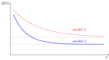
The learning curves of two online models (schematically): as objects arrive, the mean loss levels off at a horizontal asymptote. Model 1 reaches a better level faster.
The issues of incremental and online learning
By the way, what the difference between incremental and online learning is we will discuss specially a little later. For now let us consider that incrementality is when objects arrive one at a time and the model has to be updated for each object.
- How to update the model efficiently from one precedent?
- How to make the model more complex as the amount of data grows?
- How to ensure the same quality as offline?
- How to avoid storing the whole data sample?
- How to avoid "catastrophic forgetting" while doing so?
- How, while adding new objects, to remove old ones too?
What may be added in machine learning problems:
- objects, the main but not the only case;
- features;
- the dimension of the model;
- classes/clusters;
- subsamples/subproblems;
- regions of the data space, changes (concept drift).
The first question: how to update the model efficiently? This is a question of all sorts of algorithmic and programming contrivances: how to spend much less computational resource on updating the model from the one last object than on training on the whole sample from the start.
The second question is very important: how to make the model more complex as the amount of data grows? The sample grows gradually; at first it is small, and to train a model on a small sample, it should apparently be simpler: we know that the optimal complexity of a model depends on the amount of data, the more data, the more complex the model can be. So we need not only to learn to update the model's parameters when one new object arrives, but often also to decide that it is time to make the model more complex: there are now so many more data that the structure of the model can be changed, made more complex. How are these decisions to be made?
The third question: is it possible to guarantee that a model built in online mode will be exactly the same as offline? Some methods guarantee it, some do not: there are approximate methods, there are exact ones.
The fourth question: how, and is it necessary at all, to avoid storing the whole data sample? Very often the processing of stream data is arranged like this: we have updated the model and forgotten about this object altogether. We do not store the training sample: objects fly in to us, we process them, they change the model, and we throw the object itself away; we will not even have the possibility of looking at it. Things worked by such a scheme long ago, when it all began, in the 50s and 60s, when the size of a computer's memory might be one kilobyte, and there really was nowhere to store a training sample. Now it is not quite so: schemes appear for keeping some minimally necessary number of prototypes from the training sample. Hence the issue of prototype selection, and we will touch on it a little today. But if we are not going to store the sample as a whole, the effect of so-called catastrophic forgetting arises: how to build a model so that the information about past, old objects, which we do not store, is still preserved in it in some way?
And the last question, which we will not touch on today: sometimes one needs not only to add new objects incrementally but also to remove old ones decrementally. Such methods exist too, but they are something exotic.
Let us look more broadly: what may be added at all in machine learning problems? The main thing is the growth of the training sample: it grows, and the model has to be modified dynamically. This is the main but not the only case. Sometimes new features are added: the sample grows, and at some moment it was decided to measure something new; new features appeared for the new objects. As I have already said, the dimension of the model may grow.
A very important case is the appearance of new classes. For example, the problem of identifying people by their faces: if we are talking about the employees of a company, the appearance of a new employee is a new class in our identification system; it does not matter whether by face, by palm, by fingerprint or by voice. We take data from the new employee, photograph him from different angles, and it is important that the model, with the appearance of new classes, does not forget the old classes. We will talk about this a little at the end.
There are also situations where we need to solve many problems at once, a kind of multitask learning. We have already talked about such problems when we discussed deep neural networks, transfer learning and all sorts of schemes where a certain part of the network is trained common to all tasks, but each task has its own additional tuning to specific criteria, to additional data. In this case, just as in the case of classes, a problem arises: how, while extending the set of tasks we solve, not to worsen the quality of solving those tasks we have once learned? A new task appears, a certain drift, a shift happens in our models, and we must not lose the quality we have already achieved on other tasks.
That is really the whole set of issues of incremental or online learning. We will touch on most of these questions today in one way or another, but mainly we will deal with how a model is modified when new objects are added.
Online and incremental learning: what the differences are
Remark (Online Learning ≠ Incremental Learning).
- Online processes the objects in a stream, one at a time.
- Incremental may accumulate batches of updates.
- Online may forget old data (catastrophic forgetting).
- Incremental often implies the equivalence of the result to offline training on the full sample.
- Online research is concerned with theoretical guarantees.
- Incremental is focused on implementing fast algorithms.
- Online is necessarily Incremental.
- Incremental is not necessarily Online.
Let us discuss a terminological question. Very often these two terms really are used interchangeably, as synonyms. But most often online means processing the objects of a stream precisely one at a time, while incremental may mean accumulating batches of updates. For example, we have some business process, the data for a day accumulate, at night this whole batch of updates arrives, and we need to update the model. This is a rather typical situation in business applications.
Online often implies that old data are forgotten, not stored, and that very problem of catastrophic forgetting arises. Incremental often implies a proved equivalence of the algorithm trained offline and online. When you see online learning in papers, very often these are theoretical studies concerned with guarantees of quality or guarantees that the result of online learning will coincide with the result of offline learning, and so on. Incremental is a more engineering topic: it is focused on implementing fast algorithms, how to add one object and update the model, or on ensuring the equivalence of online and offline. That is, incremental is more often about data structures and algorithms, and online more often about theoretical guarantees.
And it seems that incremental is the broader notion: an online algorithm must be incremental, while an incremental one is not always online, in the sense that it may be batch. The differences really are rather fine; sometimes there is no difference at all between online and incremental, and today you will see that.
Definition (Continual learning and anytime algorithms). Continual (lifelong) learning is training one model on different tasks so that the new tasks do not displace the old ones.
An anytime algorithm is an algorithm that trains on a stream but can be used for predictions at any moment.
What else similar is there? People often speak of continual learning, or lifelong learning: training one model on different tasks so that new tasks do not displace old ones; we have already mentioned this.
And one more concept is anytime algorithms. Such an algorithm trains on a stream and keeps updating the model, but this model is always ready for use: there is another stream, when we ask the model for a forecast about a new object, and it is ready to work at any moment. It is always maintained in a current working state and at the same time keeps being updated on new data. Where is this needed? For example, in search or recommender systems, which must respond very lively, practically instantly, to changes in users' interests. We have seen that a user has begun to search for something untypical for him; we cannot wait a day to accumulate a batch of updates and rebuild the model at night. It must adjust to his interests instantly, as soon as he has begun to ask us about something new, and we must at once give him some recommendations. So the models serving users really must be incremental: there is no time to wait for the model to be rebuilt. These are anytime algorithms, which, on the one hand, keep being trained further, and on the other, are always ready at any moment to make a forecast on any object.
Lazy learning and the selection of prototype objects
A reminder: lazy learning
Enough preambles; let us get down to business and go from the simple to the complex. First we will consider methods that are very easy to adapt to the online learning scheme, and we will begin with methods of the nearest neighbour type. This is so-called lazy learning: methods that store the training sample directly. Recalling the first semester, let us name at least three such situations.
Definition (Lazy learning). is the set of stored prototypes; is a kernel of width , the similarity of a pair of objects and .
Metric classification (kNN, Parzen window, RBF):
Nonparametric regression (Nadaraya–Watson):
Nonparametric density estimation (Parzen–Rosenblatt):
The first is the nearest neighbour method. We have a training sample, and with some proximity function, let us call it a kernel, we determine which objects of the training sample are close to the object being classified, what answers these objects had, and in effect we decide by majority vote. These are metric classification methods: nearest neighbours, the Parzen window, radial basis functions.
A similar situation in regression, when we use kernel smoothing, the Nadaraya–Watson formula: to get a prediction for the object , we use a kernel and do a local averaging of the answers over the nearest objects of the training sample. All that is needed for this is to store the objects of the training sample. And the nonparametric Parzen–Rosenblatt density estimates are based on the same idea: we estimate the density at the point by how many objects there are in its nearest neighbourhood, again using a kernel.
It would seem that online is altogether very organic here: one simply has to add the new object to the stored training sample, and nothing else needs to be done, because when we compute , we simply consult the store of objects. But a specificity arises when we ask ourselves: perhaps we do not need to store the whole training sample, and it is enough to keep some subset of prototypes, or standards, as they are called in Russian?
Online prototype selection
So the scheme of online prototype selection arises. Here there is a constraint, the so-called budget: we cannot keep the whole training sample; we have an upper bound on the number of stored objects.
The first thought that comes to mind: an object has come, we classify it, for example, by the nearest neighbour method and see that it is classified poorly, so it should probably be added to the training sample; and if it is classified well, then not. This idea is in fact mistaken. Why? When we add a new object, we should pay no attention to how well it is classified by its neighbourhood. On the contrary, we need to pay attention to how much more information it adds, so that, taking it into account, the objects from its neighbourhood become better classified. One must estimate not how this object is classified, but how useful it itself is for classifying the objects that are in its neighbourhood. This idea really is sound and correct.
Definition (Online prototype selection).
- , the "budget", the maximal number of stored objects ;
- , the accumulated estimate of the usefulness of the object ;
- , a counter of how many times the object influenced another;
- , the minimal value of the influence counter;
- , the minimal influence of the object on ;
- , the loss on the object when the object is excluded from .
For all :
- get ; compute ; ; ;
- ;
- for all close to : :
- ; ;
- ; ;
- if , then .
Let us see how this is implemented in our online learning scheme. We get objects one at a time. For each object we can at once compute its classification by its neighbourhood and compute the losses, now for all the objects from the neighbourhood. Here one can impose a threshold condition on the value of the kernel. One can say that these are the objects from the neighbourhood that influenced ; but since the kernel is symmetric, it is the same as saying: let us find those objects whose classification is influenced by the added object . It does not matter how one says it; the main thing is that we look at the objects whose proximity is greater than a certain threshold , a parameter that will have to be set.
Next we estimate the loss that will occur if the object is excluded from the sample, compare it with the loss on the object , and accumulate these differences: we are interested in estimating how useful the object is for classifying the new object . For all objects of the sample these usefulness estimates are accumulated: is the total usefulness. A new object has come, and by it we have estimated how useful all the objects that turned out to be in its neighbourhood are. Besides the accumulated deltas we accumulate the counters , how many times the object was a neighbour of some other object.
By default we add the newly arrived object to the sample . Its accumulated usefulness is so far zero, because it has not yet been useful for newly arriving objects, and is also zero. Next a condition is checked: if the budget has already been exceeded, we must decide which object to exclude from the set of prototypes . We choose the object with the minimal mean usefulness, provided that it has accumulated a sufficient number of influences, ; is also a parameter of the method. If an object has been in the neighbourhood of other objects enough times and it turned out that it is not very useful, its mean usefulness is close to zero, then we boldly remove this object. The ratio is precisely the criterion by which the objects can be sorted, and the objects with its smallest value removed from the sample.
This scheme is useful not only for selecting prototypes in methods of the nearest neighbour type. It can be applied much more widely: to store not the whole training sample but its important part, at least some information about the training objects. If we forget the sample, let us forget it not entirely: let us set some budget and keep as much as we can. Similar methods can be used for prototype selection, and one such method, this time for deep neural networks, we will consider towards the end of the lecture.
Merits and drawbacks of lazy online learning
Remark (Merits and drawbacks of lazy online learning). Merits:
- simplicity of implementation;
- the solutions of online and offline are guaranteed to coincide (only when all data are stored, );
- the idea of prototype selection can be transferred to other online methods for which there is a fast way 1) to estimate the influence of some objects on others and 2) to estimate the decremental loss .
Drawbacks:
- storing the sample is not real online;
- training the window width and other parameters of the similarity functions may substantially complicate the algorithm.
To sum up: the merit of lazy online is that it is very simple, and that the solutions of online and offline are guaranteed to coincide when the sample is stored; nothing even needs to be proved here. And such ideas can be transferred to other methods.
The drawback, of course, is that if we store the whole sample, it is in fact not genuine online. If we keep only part of the sample, the prototypes, it is a very good compromise. And here too the window width has to be chosen, the proximity itself tuned somehow. This is a problem in all methods of the nearest neighbour type; we have discussed it many times; one just should not forget that the window width has to be adjusted somehow online too. By the way, it is simple to do: one should store not one proximity function but several, with different window widths. As the sample accumulates, the optimal window width will most likely adapt slightly; it may decrease: the more densely our objects sit, the narrower the proximity function that can be used.
The online naive Bayes classifier
A reminder: the naive Bayes classifier
Let us go further and think which other machine learning methods are not hard to generalise to the online scheme. Let us recall the naive Bayes classifier; it is a simple thing. When we discussed it last semester, the conclusion was this: this classifier is based simply on computing the mean values of the features for each class. And means are very easy to update by a recurrent formula when new objects arrive. I have spoiled the main idea, but to see how it looks in detail, we do need to recall better what the naive Bayes classifier is.
Definition (The naive Bayes classifier). The "optimal" Bayes classifier:
The "naive" assumption that the features are independent:
The assumption that the one-dimensional densities are exponential:
The problem of maximising the log-likelihood splits into independent subproblems over the classes and the features :
Let us begin with what the optimal Bayes classifier is. The Bayes decision rule is based on maximising the posterior probability of the class given , which can be written like this, where is the likelihood function of the class. This likelihood function is our main model. In naive Bayes it is additionally assumed that is a vector of features, and the features are statistically independent random variables. If they are statistically independent, then the multivariate density is the product of the one-dimensional densities over the individual features.
This assumption is, of course, naive. It does not always work, and one can even say that it works rarely: mostly in machine learning problems one cannot assume that the features are statistically independent. But there are applications where it works well, for example text classification, where naive Bayes is quite competitive, and it is also very fast. Why it is fast we will now figure out.
The expression under the can be logarithmised: the logarithm of a product of densities of features arises, and after logarithmising a sum of logarithms. The index numbers the features from to . When I write the index at the top, it is the index of a feature; when at the bottom, the number of an object of the training sample.
So we have made the naivety assumption. Let us make one more: the one-dimensional densities have to be modelled somehow, after all, and let us assume that they are exponential. We introduced such an assumption when we considered generalised linear models. But there the situation was a little different: there exponential densities described the 's. The method of least squares is equivalent to the assumption that the are Gaussian random variables; logistic regression arises under the assumption that the have a Bernoulli or binomial distribution. But here the assumption of exponentiality of densities is applied not to but to , and to each feature separately. Not only have we assumed that the features are independent, we also assume that each feature is described by its own exponential distribution.
What is important here? It is important that this part is linear: the product of and a model parameter. The function is arbitrary; the main thing is that it does not depend on ; the function is arbitrary; the main thing is that it does not depend on . Such is the general form of exponential densities. The beauty of this generalisation is that it covers the special cases we need most. A feature is real-valued: let us assume that it is distributed by Gauss and characterise it by its mean and variance; the variance, by the way, is expressed by the parameter . A feature is binary: let us assume that it is distributed by Bernoulli, and then there the single parameter is the probability of the value one. All these are examples of exponential densities.
The most fortunate property of exponential densities is that they allow the problem of maximising the likelihood to be decomposed. If we write out the criterion, the log-likelihood, it splits into independent subproblems over classes and over features. Why did this happen? We substituted the density under the exponential, the logarithm destroyed the exponential, a sum appeared, and we were able to swap the summation signs: the outer sums are over and over , the inner one over objects. We saw that the problems over and over are independent of each other: a decomposition has happened. To maximise this criterion, each term in brackets can be maximised separately, without looking at all the others. And this is a very simple problem, because it is one-dimensional. That is the whole beauty: the assumption that the features are independent, naive Bayes, plus exponential distributions of the features at once allow the solution to be obtained simply and in analytical form.
Exponential distributions of features
This is rather a reminder slide about why the frequently used, useful distributions we need are exponential. We take the Gaussian distribution, Bernoulli, binomial and Poisson. These are cases interesting for us, because such distributions can describe, respectively, numerical features, binary ones, integer ones with an upper bound, and features of the click-frequency type, which seem to be discrete but are not bounded above; they can be described by the Poisson distribution.
Example (Examples of exponential distributions). is the expectation parameter, the link function:
| Distribution | Values | |||||
|---|---|---|---|---|---|---|
| normal | ||||||
| Bernoulli | ||||||
| binomial | ||||||
| Poisson |
How is this to be proved? We take the expression for the distribution and show that everything can be driven under the exponential, and under the exponential a correspondence with the parameters of the exponential distribution is established. Indeed, we get a formula that falls under the exponential family. Here a connection arises between the expectation and the parameter : must multiply linearly, and it is a function of . The function also stands out automatically. Next, the derivative and the function inverse to the derivative are very useful; we will see in a moment where it will play.
The linear naive Bayes classifier
Next we have to derive the formulas for the model parameters. Since a decomposition has happened, we differentiate the log-likelihood with respect to all the model parameters and set the derivatives to zero.
Proposition. The solution for is expressed through the mean value of the feature in the class :
The solution for is expressed from the equation ; for example, in the case of the Gaussian distribution
Naïve Bayes is a linear classifier:
Online learning: recurrent formulas for , :
- speed both offline and online;
- the solutions of online and offline coincide.
What do we see? The parameter for the feature in the class is determined very simply: through the mean value of the -th feature over the objects of the class . I denote it . The function still has to be applied to it, which is why I wrote it out; but, knowing what the distribution looks like, we always know this function. It is a definite function known to us, which depends only on what assumption we have made about the form of the feature's distribution. So the solution is very simple, analytical, and the main thing is that the arithmetic mean of the -th feature for the -th class stands in it. And the arithmetic mean is very simple to compute by a recurrent formula, so an incremental algorithm is also very simple to make.
We also have the parameter , though it is not always there: if you look at the discrete-valued distributions, it is always one for them; it does not even need to be determined. And for the normal distribution it is simply the variance, , and for the variance there are also efficient recurrent formulas: how to recompute the sample variance if one more object has been added. I will not even give this formula; it is very simple.
In the end naive Bayes turns out to be a linear classifier. It is clear why linear: we took the logarithm of the density, the logarithm destroyed the exponential, and enters only linearly. also enters the function ; but if does not depend on , it can be removed under the ; we do not need it at all, and it is often simply thrown out. It does not depend on if we determine the parameter in such a way that it is the same in all classes. And everything else is simply the coefficients of the linear model and the intercept . So we have ready formulas to compute all of this.
The online naive Bayes classifier (ONB)
What did we recall all this for? To show that the online naive Bayes classifier is very simply implemented in our general scheme, when the objects arrive one at a time.
Definition (The online naive Bayes classifier (ONB)).
- Initialise ; ; ;
- for all :
- get the next object ;
- make a prediction ;
- get the answer and estimate the loss ;
- for update the means by the recurrent formula: ; ;
- estimate the parameters of the distributions: and (depending on the type of the feature);
- update the coefficients of the linear model: ; .
We get the next object, make a prediction with our linear classifier, get the answer, estimate the loss, and now we update the arithmetic means by the recurrent formula. Here it is, the recurrent formula: how to update the mean value of the -th feature for the -th class if one more object has appeared; we take the value of this feature from it. A very simple formula. Next we estimate the parameters of the distributions by the ready analytical formulas and update the coefficients of the linear model. That is all.
So the naive Bayes classifier is simply a linear classifier in which the coefficients are computed by analytical formulas. For this computation we must know from which exponential family the given feature is taken. The assumption of a specific exponential distribution simply gives us a way to compute the model parameters from the mean value.
Merits and drawbacks of ONB
Remark (Merits and drawbacks of ONB). Merits:
- speed both offline and online;
- the solutions of online and offline coincide;
- insensitive to the number of classes and to class imbalance;
- practically never overfits;
- suitable for heterogeneous data and data with missing values;
- in text classification problems the quality is comparable to SVM (when feature selection by TF-IDF is introduced);
- often used as a "baseline to beat".
Drawbacks:
- in most problems the "naive" assumption that the features are independent does not work at all.
J. Rennie et al. Tackling the poor assumptions of Naive Bayes text classifiers. 2003.
The first merit is linear computational complexity. This is great: one can compute very fast, both online and offline; essentially nothing has to be done here except computing arithmetic means. The second: the solutions online and offline coincide, unless, of course, we have accumulated some computational errors in the recurrent formulas for the means.
The method is very insensitive to the number of classes and to class imbalance and practically does not overfit. Why? By the law of large numbers: the parameters of this method are computed as arithmetic means, and if you have split the sample into train and test, randomly at that, the arithmetic means will be very close to each other. Unlike linear models such as SVM or logistic regression, where one has to fight multicollinearity in a special way and invent regularisation, nothing of the kind is needed here: naive Bayes does not suffer from multicollinearity at all, because the assumption that the features are independent is built into it.
The method is well suited to heterogeneous data: one simply has to introduce for each feature its own assumption about the exponential family, and the features can be continuous, discrete, binary, anything at all. It also copes well with missing values: if some feature has not been measured in an object, we simply ignore it when computing the arithmetic means; nothing else needs to be done.
Because of its speed this method is often used as a baseline. If some methods have to be compared with each other, it is a good idea to take naive Bayes. Its quality is, as a rule, worse, and beating it is not such a hard task; it gives approximate values of the quality criteria, a kind of lower bound. It is hardly worth making methods worse than naive Bayes; one should try to improve on it.
The drawback, of course, is that the naive assumption that the features are independent does not work in many problems, not at all. The most successful application, as I have already said, is text classification, especially if competent feature selection is done as well. The features in a text classification problem are in effect word frequencies. If the coefficient of a feature in naive Bayes is close to zero, it should be dropped; selection can also be done in different ways, by TF-IDF for example. If a word occurs about equally often in different classes, it is probably uninformative and can be thrown out. Naive Bayes with such feature selection is in general very successful and sometimes even competes with SVM, which is considered the state of the art in text classification problems. So, naive as it seems, in some problems it works quite well.
We have considered two classes of methods: lazy learning with prototype selection and the naive Bayes classifier. It may have been hard here, because perhaps not everyone remembers what exponential families are. Today we have considered one more way of applying this very useful device: whereas in generalised linear models we described the 's with exponential densities, now I have shown how to describe the 's and how to use it in an incremental scheme. By the way, it is clear that naive Bayes with exponentially distributed features can be used not only online: everything works in exactly the same way in the ordinary offline scheme, when we train on the whole sample at once.
Gradient methods
The Perceptron algorithm
Let us begin with a couple of methods that are rather of historical interest, because that is where it all once began. I refer to Frank Rosenblatt's paper of as long ago as 1958: these are the first attempts to build neural networks, the perceptron. Back then the power of computers really did not allow samples to be stored; very many methods worked just like that, and there were many different heuristics for how to update the model parameters when the next object arrived and forget this object for ever.
Definition (The Perceptron algorithm for a linear classifier). Let , ; the model .
The oldest online learning algorithm (Hebb's rule):
- initialise the model parameters ;
- for all :
- get ; predict ; get ;
- if , update the model .
This is equivalent to a gradient step with the loss function and step size .
The variant with normalisation: .
Frank Rosenblatt. The perceptron: a probabilistic model for information storage and organization in the brain. 1958.
Let us begin with a linear classifier: it really is the perceptron. There are two classes, and , and the model is arranged as the sign of the scalar product of and . This algorithm is probably the oldest online learning algorithm altogether and perhaps one of the very first machine learning algorithms in general.
The objects arrive one at a time: we get an object, make a prediction, get the answer and do a very simple thing. If the answer did not coincide with the correct one, we update the model by simply adding the object's vector with a sign to the weight vector: if the correct answer was , we increase by , and if was , we subtract the vector from the vector . That is how the update is arranged.
Originally this heuristic appeared as the result of certain reasoning on a neurophysiological theme: about how real nerve cells work and how they consolidate their learning. But later it turned out that it is much simpler to interpret this algorithm as a stochastic gradient method. This heuristic turned out to be simply equivalent to a gradient step if one takes such a loss function and does not adapt the step size: the gradient step, which we usually denote , is simply equal to one. It is clear that the gradient step can be tuned too, and a cleverer loss function can be taken; but nevertheless the very first algorithm, the perceptron, in fact performs gradient optimisation.
There is also a variant with normalisation. This loss function is similar to the SVM one: it is also called hinge, piecewise linear, of two pieces. But it has no one: in SVM there is , while here there is minus the margin, and the one is missing. In SVM the loss function is much cleverer, although it seems to differ only by this one: it begins to penalise objects for approaching the boundary between the classes and thereby tries to build the separating surface so that the classes stand as far from it as possible. This principle helps very much to raise the quality of classification, but when the perceptron was invented nothing was known about it yet.
Loss functions of the margin : the threshold , the perceptron (Hebb) and the hinge (SVM) (slide).
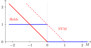
Loss functions of the margin : the threshold (blue), the perceptron (Hebb) and the hinge (SVM, dashed).
The Passive-Aggressive algorithm
The next algorithm is not so old, but in essence very similar. It is called Passive-Aggressive; it is also a linear classifier, but now we take the loss function as in SVM, with the one.
Definition (The Passive-Aggressive algorithm for a linear classifier). is the loss function as in SVM.
The idea: is the projection of onto the set :
- passive: if , do not change the weights, ;
- aggressive: move as far as possible towards .
The problem of finding the point with the parameter and the power :
The analytical solution gives the value of the gradient step :
K. Crammer et al. Online passive-aggressive algorithms. JMLR, 2006.
The idea is to correct the vector in such a way as to project it onto the set of those for which the loss is zero. What is this set? It is the set of such as correspond to the right branch of the loss function, where it is zero. If an object has come that falls into this right zone, the loss is zero, and then we do not update the weight vector: we react passively to the appearance of this object. If an object has come on which we have a non-zero loss, we try to move the vector in the direction of decreasing the loss function, and aggressively, as far as possible.
How do we pose this problem as an optimisation problem? We seek the new value from the solution of such a problem. On the one hand, we minimise the loss on the object that has just come to us; here the loss is also raised to the power , a parameter of the method. On the other hand, we strive not to go too far from the previous value : this is a kind of regularisation; it tells us that one may not jump too far from the current approximation of the parameter vector.
Such a small optimisation problem can be solved analytically, and the analytical solution leads everything to the same perceptron rule and gradient method. What was once invented from neurophysiological considerations, and all this, are very similar things. Only here a formula for the gradient step is obtained: it arises as the analytical solution of the optimisation problem. One can differentiate it with respect to , set the derivative to zero and express from it; it turns out that this is a certain shift from the current vector . Depending on how we take , different formulas for arise. For more detail, see the paper on the online Passive-Aggressive algorithm.
Online gradient descent
All these are special cases. Let us now consider the general case, when we minimise an additive criterion and the objects come to us one at a time.
Definition (Online Gradient Descent (OGD)). Minimisation of the additive criterion
The difference from the SGD method (Stochastic Gradient Descent) is that the objects follow in a given order, not in a random one:
- initialise the model parameters ;
- for all :
- get the object ; predict ;
- get the answer ; estimate the loss ;
- update the model .
M. Zinkevich. Online convex programming and generalized infinitesimal gradient ascent. 2003.
In effect we do practically the same thing that you already know as the stochastic gradient method, only here it is called online gradient descent. What is the difference between stochastic and online? In stochastic we take the objects of the training sample in random order and walk over the sample in circles, so that each object may be chosen many times. Here we have no such possibility, and we simply take the objects in the order in which they arrive to us in the online process.
We have got an object, made a prediction with the current parameter vector and, having got the correct answer, estimated the loss. Now for the new object we have both and , and we can use them to update the model's parameter vector. That is what we do: we make a gradient step; I have not written out the gradient of the loss function with respect to the parameter vector. Next one has to decide which specific loss function we take for our specific problem, and this is a general recipe.
Sometimes this is also called online convex programming. In general, online methods of the gradient descent type have been studied very intensively over the last couple of decades, and very many different interesting modifications have appeared. Let us not go into these technical details. What matters to us now is the idea: online gradient descent is simply the twin brother of stochastic gradient; they differ only in the order in which the objects are processed.
Online gradient descent is very good in that it is precisely this method that is used to train neural networks. If we want to train a neural network in online mode, we apply this method, and it differs little from the ordinary stochastic gradient descent usually used to train neural networks. So making online training of a neural network is a very simple thing. Well, almost; we will come back to this at the end of the lecture.
The recursive least squares method
Let us see how other machine learning methods are modified when new objects are added. Let us take the least squares method: today is a day of memories of the first semester. Let us recall how multivariate linear regression and the least squares method are arranged.
Definition (The least squares method and the Sherman–Morrison formula). Let , ; the regression model .
The least squares method (LSM) for linear regression:
The solution of the LSM problem (ridge regression):
The new object is appended as the bottom row of :
The Sherman–Morrison formula for the matrix :
The regression model is the scalar product of the object's feature vector and the model's parameter vector; are, naturally, real numbers. The least squares method is the sum of squared residuals between the model and the correct value , and we add regularisation at once as a way to fight overfitting and multicollinearity; is the regularisation coefficient. This is called ridge regression. We minimise such a functional over the vector ; is the "objects–features" matrix: the rows correspond to objects, the columns to features.
If we add one more object to the training sample, one more row is appended to the matrix at the bottom, and one more value is also appended to the vector at the bottom. We must be able to recompute the solution of the problem in this case. We know the solution of the problem: it is the well-known ridge regression formula, and you derived it last semester. If is zero, the highlighted matrix is called the pseudo-inverse; in the general case with the problem can be solved by applying SVD, the singular value decomposition; we considered this too.
But now we have a different situation: we add objects to the training sample one at a time, and the new object is added as a bottom row. Let us write what the matrix will look like in this case, in block form. We have added a row at the bottom of the matrix and found that at every iteration we must add to the matrix a matrix of rank 1, , the product of a column and a row.
It would be very nice to have an incremental formula: if the inverse of the matrix is already known, how to compute the inverse of the matrix obtained by adding one row to at the bottom? Fortunately, there is a well-known Sherman–Morrison formula for this problem: if we have a matrix and its inverse is known, here is how to compute the inverse of the matrix . The Sherman–Morrison formula gives a slightly more general representation, with , while we have the special case , and we can simply use this formula.
I note also that I have added at once, the ridge that comes from the regulariser. It can be added from the very beginning: when we have no objects at all, we know that we have features, and we start with the matrix , whose inverse is very simple to find. The first object of the training sample has been added, and we can already compute the inverse by the Sherman–Morrison formula. This is quite remarkable: with such incremental computation one can, generally speaking, train the least squares method. Up to the accumulation of computational errors, the Sherman–Morrison formula guarantees that, having looked through all the objects of the training sample once, we will get that very inverse matrix, which remains only to be multiplied by , and we will get the ridge regression solution.
Definition (Recursive Least Squares (RLS)).
- Initialise , ;
- for all :
- get the object ; make a prediction ;
- get the answer ; estimate the loss ;
- ;
- .
Complexity ; the solution is exact and coincides with offline.
Comparison with OGD:
Complexity ; the solution is approximate and differs from offline.
Here I set this out as an algorithm. Such an approach is called the recursive least squares method. Even if our problem is not online, it can simply be used to compute the solution of a least squares problem. It gives slightly less information than SVD: there are no eigenvalues here, no understanding of how much they differ, so as to estimate how strong the effects of multicollinearity are. But nevertheless, for a fixed the solution of the ridge regression problem can quite well be computed by such formulas.
The scheme is the same as usual in our online algorithms: we get an object, make a prediction, then get the correct answer, estimate the loss and update the inverse matrix by the Sherman–Morrison formula. Here is already , that is, we compute the inverse matrix at once from the inverse matrix for the previous sample, smaller by one.
What is the complexity of this algorithm? It is easy to compute that it is . Why? The Sherman–Morrison formula has a computational complexity of order : here we are multiplying a matrix by a vector of dimension , that is , and we do this times, as many as there are objects in the training sample.
It is interesting to compare this formula with online gradient descent: it turns out that they are madly similar to each other. The only difference is that in online gradient descent there is multiplication by a scalar here, the gradient step, while here there is multiplication by a matrix. Of course, this takes longer: here the complexity of a step is , while in gradient descent the complexity of each step is . But gradient descent is an approximate method. If we could use stochastic gradient descent, we would start repeating these steps many times, looking through the sample, and the process would go on converging. In the online method we cannot afford this: we will also make exactly steps, but the solution will be approximate. And the recursive least squares method is an exact method: it guarantees that the solutions of online and offline coincide, and only exactly steps need to be made.
Although, of course, one can store the training sample or part of the objects, select prototypes, and then make further gradient steps on them. Such methods exist too, but I will not consider them here, because it is yet another modification of the online gradient descent scheme.
Remark (Does online coincide with offline). In the recursive least squares method there is essentially no difference compared with offline: we simply feed the objects in turn into the Sherman–Morrison formula. If no computational error accumulates, then, purely mathematically, the result must coincide with the offline one.
Incremental decision trees
One more case for which an incremental analogue is known and the identity of the results of online and offline is also guaranteed is decision trees. First I will recall what a decision tree is and how the ID3 algorithm is arranged in the ordinary, offline formulation.
A reminder: the decision tree
Definition (Decision Tree). is the set of features, , .
A decision tree is a classification algorithm given by a tree (a connected acyclic graph):
- , is the root of the tree;
- : a feature and a function ;
- : a class label .
Classification of an object : ; while : ; output .
If for all , the decision tree is binary.
We have a finite set of features, of them, and for simplicity let us consider them binary. Each feature has its own set of values; here I denote it ; if it is a two-element set and all the features are binary, we will have a binary decision tree, as shown in the picture.
A decision tree is a connected acyclic graph. There is a single root vertex, denoted , and vertices of two types: internal and leaf. Internal vertices have children. An internal vertex stores, first, a feature and, second, a function which, from the value of the feature, points to a child vertex. Leaf vertices store class labels.
When we need to classify an object, we start from the root of the tree and get to a leaf in this way. While we are at an internal vertex, we compute the value of the feature ; the value of the feature at this internal vertex indicates which child vertex we need to take next, and we pass to this child vertex. We make transitions in this way until we run into a leaf vertex, in which we simply take the ready answer, the class label.
A binary decision tree: from each internal vertex the value of the feature points to the child vertex or (slide).
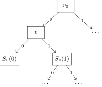
A binary decision tree: from each internal vertex the value of the feature points to the child vertex or .
A reminder: the ID3 algorithm
The next reminder slide is how to train a decision tree with the ID3 algorithm. The abbreviation stands for Iterative Dichotomiser, iterative splitting of the sample. The word "iterative" here is not quite in our sense: there is no incrementality over objects in this algorithm.
Definition (The ID3 decision tree learning algorithm). ; the function calls itself recursively.
The function the root of the tree :
- , the branching criterion of the tree;
- if , create a new leaf ; ; output ;
- create a new internal vertex with the function ;
- for all : ; ;
- output .
The majority rule: .
John Ross Quinlan. Induction of Decision Trees // Machine Learning, 1986.
Let us see how this function works. It is recursive: it takes a sample as input and returns the root of the tree built on this sample. Suppose the sample has come as input. First of all we look for a feature that can split this sample so that we get the maximum gain from classifying the two parts of the sample separately. How this gain function is arranged I will not say now: we went through it in some detail in the first semester; information gain, the Gini criterion, one can use entropy or something in that spirit. It does not matter now.
The main thing: if we could not achieve a good gain, we create a new leaf vertex and, by the majority of the objects that came to this vertex, decide which class it will correspond to; this is the majority rule. If, however, we do manage to get a sufficiently substantial gain by splitting into child vertices, we split the sample by each value of the feature : the sample is divided into subsamples by the value that the feature chosen for the vertex takes on the object. To each such subsample we apply the function : it calls itself recursively, but on a sample of smaller size, and returns the root of the tree optimally built on this subsample. It only remains for us to attach this tree as a child vertex to the internal vertex just created.
That is how this thing works. But I note that there is no incrementality over objects here at all. Moreover, implies that we compute, usually, a sum over all objects of the sample : the sample , and hence the whole sample , must be given initially, known and fixed, so that we can split it into subsamples and compute these very on each subsample.
The incremental ID5R algorithm
The question: if a new object is joined to the sample , how will this algorithm change? In fact it changes in an absolutely radical way: an algorithm that trains decision trees incrementally is arranged quite differently. Such an algorithm was invented by Paul Utgoff. He had about a dozen publications; year after year he gradually improved these algorithms; he worked on this for ten years, probably. One of the algorithms, called ID5R, guarantees that the trained decision tree will be exactly the same as the one obtained by the ID3 algorithm.
Definition (The incremental ID5R decision tree learning algorithm). is the set of objects that have reached the vertex ;
are counters of the number of objects for computing the branching criterion .
For all :
- get ; predict ; get ;
- for all on the path from to the leaf has fallen into:
- for all ;
- , the branching criterion;
- if and , turn into an internal vertex;
- if and , then ; .
Paul E. Utgoff. Incremental Induction of Decision Trees. 1989.
What is the idea here? The most important idea is that every vertex of the tree will have to store such counters: in effect a three-dimensional array of integers, the number of sample objects that have reached the given internal vertex . We pass all the objects of the sample through the tree, and at every internal vertex a subset forms of the training objects that have reached this vertex. Now this subset will begin to expand, since new objects are added to the sample, and the information about the whole previous sample will be stored in these counters.
Such a three-dimensional array counts the number of objects, among those that reached this internal vertex, with a given value of and a given value of the -th feature. The feature is not fixed: for all features from to we will store the number of objects that have the class and at the same time the value of the given feature, where runs over all possible values of the -th feature. It seems a huge three-dimensional array, but in fact it is not so huge. If, for example, we have a binary classification problem and all the features are binary, the volume of stored data is only : two possible values for , two possible values for , four values in all for each of the features. That is not wildly much. Of course, if there are many classes and the features are many-valued as well, a game begins of how to store this array more efficiently.
That is the main invention: to store such a three-dimensional array at every internal vertex. After that everything is relatively easy; relatively, because I will not tell certain technical details. As usual in the online scheme, we get an object, make a prediction, get the correct answer and begin working on how to rebuild the tree. First, we pass the object along all paths in the tree from the root to a leaf vertex, simply because we do not yet know which feature will finally be chosen at each internal vertex. The counters leave, as it were, the possibility for any feature to be chosen for the given vertex. And the main thing: as the tree grows, the feature at each vertex may change with the growth of the number of objects in the training sample.
So for all internal vertices we update the values of the counters for all features. If we have these counter values, we can compute for any feature from them. That is the answer to the question why it is precisely such a three-dimensional array that must be stored: it allows to be computed at every vertex for all features and the feature chosen that will now be the optimal branching criterion at the given vertex. Next come the rules that are applied either to turn the given vertex into an internal one, or to restructure the subtree that now sits at this internal vertex. How exactly the subtree is restructured I will not explain in detail: there are many programming subtleties there. Whoever is interested can look at the paper on how it is implemented, or use a ready implementation. The main idea of this method is to store such three-dimensional arrays at every internal vertex of the tree.
Remark (A one-pass algorithm). Does the algorithm not run through all the data anew when a new object comes? No: this algorithm is precisely incremental. It passes through the sample once and, as it goes, creates new vertices and grows the tree. This is an example of an algorithm in which the structure of the model becomes more complex gradually, as the training sample grows, and it is a one-pass algorithm: all the logic here is one loop over the objects of the sample. Its complexity is not much greater than that of the ordinary ID3: from time to time subtrees have to be rebuilt, but this does not take too much time.
Remark (Merits and drawbacks of ID5R). Merits:
- counters are stored, not the sample;
- the tree grows gradually as the amount of data grows;
- the solutions of online (ID5R) and offline (ID3) coincide.
Drawbacks:
- a large volume of stored data;
- because of this a large forest of ID5R is hard to build.
P. E. Utgoff. An improved algorithm for incremental induction of decision trees. 1994. P. E. Utgoff, N. C. Berkman, J. A. Clouse. Decision tree induction based on efficient tree restructuring. 1996.
The main feature of this algorithm is that it has been proved, and the theorem is not very simple, that the result of training ID5R is the same as that of ID3. True, at once a heap of heuristics arises on the theme of "let us do pruning", and pruning may already change the result of training. So ID5R is, after all, building a decision tree without pruning; if pruning is done, the scheme changes somewhat, and there will no longer be a guarantee. But, in general, guarantees that the result will coincide with ID3 with pruning, for example, are not really needed.
Online training of ensembles: the Hedge algorithm
The Hedge(β) algorithm
Let us go further; there is still much of interest ahead. Two classes of algorithms remain, but very important ones: the first is compositions, the second neural networks, deep ones included. To begin with, I want to tell you about the quite remarkable Hedge algorithm, invented by the authors of boosting, Freund and Schapire: they worked out how to make boosting incremental.
Definition (Online training of an ensemble: the Hedge(β) algorithm).
- , , the [trainable] base predictors;
- , a loss function convex in ;
- , the parameter of the base of the power ( decreases in ).
In boosting we fix and grow , while in Hedge it is the other way round!
- Initialise the weights of the predictors , ;
- for all :
- get the next object ;
- make predictions , ;
- get the answer and estimate the losses ;
- update the weights of the predictors: ;
- further train the predictors , on .
Here is the normalisation of the weights to unit sum over .
Yoav Freund, Robert E. Schapire. A decision-theoretic generalization of on-line learning and an application to boosting. 1997.
The formulation of the problem: we have certain base predictors, which may be either trainable or not trainable. The problem is very similar to the one we considered at the end of the last lecture, compositions of forecasting algorithms; the situation is very similar. There is a loss function convex in ; why convexity is needed we will understand in a couple of slides; for now we simply assume that for a given base predictor, having the correct answer , we can estimate the loss. A parameter from zero to one is set, and note that the power function for less than one decreases in ; this will be useful to us.
The main difference from boosting is this. How does boosting work? We have a training sample of fixed length , and we grow the base algorithms: is fixed, while is all the time increased by one; we add new and new base algorithms until we see that we classify the sample very well. Now we need to pass to the reverse scheme: we have a fixed number of base algorithms, while the size of the sample grows by one at a time. This change of logic is the main difference of this method from boosting.
Let us see how this looks in our online scheme. To begin with, we must initialise the weights of the predictors. We do not know which predictor is better and which worse, so we initialise them equal. Let us agree that our weights will be normalised: over the vector sums to one, and the weights are non-negative. Then the objects begin to arrive to us one at a time. For each object we make predictions with all the predictors, get the correct answer and estimate the losses for each predictor; let us denote this loss , the loss the predictor number had on this object.
Now the most interesting part: we update the weights of the predictors. We multiply the weight the predictor had by to the power of the loss. What does this mean? decreases in , so the greater the loss, the smaller the weight of this predictor will turn out: the more a predictor errs, the smaller the weight it gets in the end. And we renormalise all these weights over , so that is all the time maintained as a discrete distribution over all the base predictors.
The last step: if the predictors are trainable, we can train them further on this new object. That is, the predictors themselves may be online machine learning methods, or they may be simply some fixed features without any parameters at all. In this method it does not matter whether the base predictors are trainable or not, and this too is a very important generalisation of boosting: in boosting the base algorithms are always trainable. The authors went down the path of extension, proved a certain very important theorem, and it turned out that for the proof it does not matter at all what the base predictors are.
The financial interpretation of the Hedge(β) algorithm
Here the question may arise why the algorithm is called Hedge. I asked myself this question, because I have an answer prepared for it. It is a very amusing paper: the authors called their algorithm Hedge, but in the whole paper it is mentioned only once, in passing, that this algorithm can be applied to playing the stock exchange. Hedge comes from "hedging", hedge funds; this is the terminology of portfolio investors.
There is a problem called online portfolio selection, and there is a separate stream of publications on it. It is about how to redistribute capital over financial instruments that keep changing their returns, and how to diversify a portfolio so as, on the one hand, to reduce risks and, on the other, to invest capital in those instruments that are the most profitable. You probably feel that the portfolio selection problem is very similar to the formulation of the online machine learning problem in which we train base predictors.
Theorem (Freund, Schapire). The portfolio investor's problem (Online Portfolio Selection):
- , financial instruments or strategies (equity);
- , the loss from the instrument at the moment of time ;
- , the share of capital in the instrument at the moment of time ;
- , the loss over the whole portfolio at the moment .
For any the loss of the ensemble is not much worse than the loss of the best of the predictors and tends to it as :
Interpretation: the return of the portfolio tends to the return of the best of the instruments as at the rate .
The base predictors are in effect our equities: financial instruments, shares, bonds or some ready strategies. The main thing is that for each of them at any moment of time we can compute the loss. The loss is, for example, minus the return, or we can define the loss however we like. The weight is interpreted as the share of capital we have put into this financial instrument at the moment of time . That the weights are normalised over is very important for us, because these are literally shares of capital: they must sum to one. This is how you redistribute capital over the base financial instruments, that is, the composition of the portfolio. And we can easily write the loss over the whole portfolio: if is the loss from the given financial instrument, and the share of capital is in this instrument, then shows the total loss over the whole portfolio.
So, the brilliant theorem of Freund and Schapire says that, however the losses are distributed, this whole matrix of size by the length of the training sample, the losses of the ensemble are not much worse than the losses of the best of the predictors. What made this possible? The fact that there is a special formula which says: if a base predictor's losses are large, its weight must be reduced. Only by virtue of this rule can an upper bound on the mean loss be proved, and it turns out that the losses of the ensemble, that is, of the whole portfolio, are not much worse than the losses of the best of the predictors. Here there is a minimum over , the best. We do not know in advance which will be the best; everything keeps changing all the time; but it turns out that if we redistribute capital over the portfolio in this way, we play not much worse than if we had known in advance, for the whole game ahead, which predictor or which financial instrument would be the most successful.
The additional terms are called regret: we do work a little worse than the very best predictor. But this "a little worse", fortunately, tends to zero as the number of objects grows, and objects for us are time. The longer we play on the market with our algorithm, the smaller our regret: on average we play like the very best instrument in the whole portfolio. Such is the financial interpretation, and in effect a ready tool for portfolio investors with a ready theoretical proof that it works quite well.
Remark (Can one get rich this way). Was this really used in practice? Can one make a player who will literally predict share prices? First, such algorithms and dozens of their modifications are used: online portfolio selection is a rather well-developed topic, and the peak of its popularity was some 15–20 years ago; there were very many publications then, and this publication of Freund and Schapire was absolutely in the spirit of this direction of research. But they say this about it: as soon as someone publishes a strategy, it stops being a winning one. Many market players, having learned of it, begin to use a similar strategy, and the more players use a successful strategy, the smaller the gain of each. As a result, the public availability of successful strategies cancels out their success: it is smeared over a large number of market players, and they have to invent something else, look for other arbitrage opportunities. So when algorithms of this kind appeared, for a while they worked quite well, but then very quickly stopped working, precisely because many people learned of them.
Properties of the Hedge(β) algorithm
Let us return to machine learning and to our original formulation, where we have base predictors. What can we say about such a combination; how well will it work?
Remark (Properties of the Hedge(β) algorithm).
- The theorem holds for any , without any probabilistic assumptions.
- The same bound also holds for the mean losses of the ensemble, by virtue of the convexity of the loss function and the normalisation of :
- The smaller , the faster the ensemble learns.
- can be estimated by minimising a more precise bound:
I draw your attention: although in form this result somewhat resembles the laws of large numbers and the convergence theorems of probability theory, not a word was said anywhere here about probabilities. No probabilistic models were brought in here, although in form the result is very similar to a probabilistic one. This theorem holds for any bounded loss function. It is a quite wonderful result. Quite a lot of such results are known by now: they do not rely on probability theory, but they allow one to prove that asymptotic results of this kind hold.
We do still need to use convexity a little to prove that the loss of the ensemble is also bounded above. Note that the bound in the theorem is given for , the mean loss on the -th object over the whole ensemble, that is, a sum in which we weight the losses of the individual base predictors. But we need a somewhat different quantity: in fact we want to estimate the loss of a convex combination of base predictors, while we have been given an upper bound for a convex combination of loss functions. But no problem arises if we take precisely convex loss functions: by virtue of the convexity property, the quantity we need is bounded above by the quantity bounded by the theorem. All is well: for our convex combination of base predictors there is also a guaranteed theoretical result.
One last question remains: how to find the parameter ? It is clear that the smaller , the faster the weights will change, and the larger , the slower. Somewhere there is a golden mean: the weights must change neither too fast nor too slowly. The optimal can indeed be estimated by minimising a more precise bound for the sum of . This formula was derived in the paper as an intermediate one; then it was slightly simplified and the more elegant analytical formula in the theorem was obtained, but it is an overestimated bound. One can optimise by the bound that is not overestimated; such an optimisation can be done numerically and the value of the parameter obtained for each specific problem. This is not hard to do.
Online deep learning
An ensemble of classifiers over the layers of the network
Now let us take up neural networks; the last piece is about deep learning: how, then, are deep networks to be trained in online mode? It would seem that I have already answered this question when we considered online gradient descent: I said that it is almost the same as stochastic gradient. But I did not mention then the main problem that arises.
Suppose you are going to train a deep neural network of a certain architecture and have already set how many layers you want and some number of neurons in each layer, quite a lot. The question arises: if there is no training sample yet, or it is small, how are you going to train this huge architecture? And the network must work not only after you finish the training process, otherwise there is no point in online. Suppose somewhere in the future you will have a million objects; but when you have got only the first thousand of them, your neural network must already be working. Even if you have got only 30 objects, the network must already work: you have no time to wait until a million objects are fed in. That is online. And the question is how to ensure that the neural network becomes more complex gradually. You want it from the start to have, for example, 10 layers of 100 neurons each; but if there are 30 objects in the training sample, it is clear that you will not be able to train this whole structure adequately. And we want everything to work as well as possible: as well as one can learn from the 30 objects, or the thousand, we have already had. How is this to be done?
Definition (Online deep learning). A network for multiclass classification with layers, :
The problem: how to train all the layers while there are few data?
After each layer we will build a classifier :
and a linear ensemble with weights :
D. Sahoo et al. Online deep learning: learning deep neural networks on the fly. 2018.
Let us consider the multiclass classification problem; whether the network is fully connected or not does not matter: with the structure of the matrices you can describe the architecture of the connections between the layers. How is this neural network arranged? As usual, the layers are written one after another, is the activation function, linear neurons, and at the end there is a softmax with yet another parameter matrix . That is, in effect, the output of the last layer is an embedding, and, to solve the classification problem further, is fed to the input of a multiclass classifier through softmax, and on we then impose some loss function, log loss or something else. It is important to remember that is an embedding, that is, new features in the description of the object , by which we can solve the multiclass classification problem.
How is it proposed to solve the problem that, when there are few data, we are not able to train all these layers adequately? The idea: when there are few data, we will use only the results of the first layers. Let us apply an analogue of this softmax straight away over the original objects: we take softmax not only after the last layer but after each one, and even after the zeroth. is the original description of the object, and we can already feed to the input of softmax; this will be an ordinary single-layer perceptron for multiclass classification for us. That is, after each layer we in effect get the possibility of classifying our objects.
Let us make a composition of the outputs of these intermediate classifiers. The first classifier is based only on softmax over the original objects. The second builds the first layer, makes a softmax over it and is based on the embedding , on the new features in the description of the object. Next, from this feature description one can make , that is, a two-layer network, and again make a softmax layer and get one more classifier. We have as many such classifiers as there are layers, plus one: we have also built a separate classifier on the original feature descriptions. Over these classifiers let us make a linear ensemble with weights.
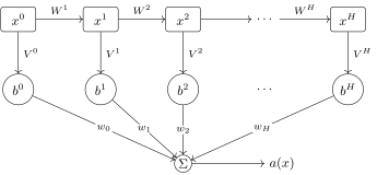
Online deep learning: after each layer a classifier of its own is built, and the answer of the network is their linear ensemble with weights .
Backpropagation: Hedge BackProp
To determine these weights, let us apply that very Hedge we have just considered, the good old Hedge of Freund and Schapire. That is, we will train the weights not by backpropagation but by the Hedge algorithm, and, accordingly, we do not need backpropagation for these weights.
Definition (Hedge BackProp).
- The ensemble weights are computed by the Hedge(β) algorithm.
- The loss function is the multiclass log-loss:
- The specifics of the gradient steps in OGD:
- Hedge switches the layers on gradually as the amount of data grows.
D. Sahoo et al. Online deep learning: learning deep neural networks on the fly. 2018.
The loss function may be any, for example the multiclass log loss. The specifics of the gradient steps are that they take this architecture into account. First, is used here not as a parameter of the neural network but simply as a ready coefficient that we get from the ensemble; the Hedge algorithm supplies it. So here it comes out as a multiplier of the gradient step. All we need to learn to do is to pass the gradients through this neural network architecture, to determine the network parameters and .
They differ, by the way, in this amusing summation. It means that to train we need to know how the following embeddings did: and so on, up to . We pass the gradient to train , and is in effect trained over all the classifiers from to .
The most interesting thing is to look at how the coefficients are distributed in the Hedge algorithm as we increase the size of the training sample. The whole method was proposed in a 2018 paper, and such plots come from there. The network in the experiment had 20 layers. We have looked at half a per cent of the data and see: about 70 % of the weight is concentrated on the classifier that uses only the original feature description. We have not yet gathered enough data to train a deep neural network architecture, so only the very first classifier, , works. But the Hedge algorithm is built in such a remarkable way that it assigns large weights to classifiers as soon as they begin to work properly. When we have looked at 10–15 % of the data, one sees that the most successful is already the third layer, a three-layer neural network; and at 60–80 % of the data, a four-layer one.
These neural networks are, as it were, nested in one another: each next one takes as input the embedding the previous one produced. At the same time they are trained together, and the most reliable classification result is determined by the Hedge algorithm. And the 20 layers originally built into the architecture here are a provision for the future: one can increase the amount of training data a hundred times more, the maximum of the weights will slowly creep to the right, and this will mean that our reserve of architectural richness, this very 20-layer neural network, is still sufficient. We get the optimal results somewhere with a 4–5-layer network, and that is how the weights of these networks are distributed.
Such is the remarkable approach that can be used to make deep neural network architectures implicitly deeper and deeper as the size of the training sample grows. We have set the original architecture, but as the sample grows, a larger and larger reserve of parameters is used in this architecture; one could say, a larger and larger number of degrees of freedom.
Remark (Will the model overfit on the stream). If data arrive endlessly, a little at a time, could it be that a tree, a regression or a simple neural network at some moment begins to overfit? First, nobody is insured against overfitting. Second, overfitting usually decreases as the data grow, rather than arising. Here Hedge is aimed precisely at suppressing the superfluous layers, which simply cannot be trained well on a small amount of data. It understands that these are bad classifiers: the first layer is good, it could be trained on a per cent of the data, while all the others are bad, and it has suppressed them. As the training data grow we begin to understand which layers are more successful, and this happens automatically through using Hedge as a tool for ensembling the results from all the layers. The higher layers are practically switched off; Hedge itself has determined which layers must be switched off, and as the sample grows they will gradually be switched on, and no overfitting will happen. Besides, overfitting can also be fought by various known devices: include a regulariser, dropout or something else in training the neural network. Nobody forbids this; it can quite well be fitted into the whole scheme.
Incremental learning of new classes: iCaRL
The formulation of the problem
One last story remains, but it is the most interesting: how deep neural networks are to learn under conditions where new classes keep arriving. Here incrementality is not only in the sense that the number of objects of the training sample grows: these objects may also belong to new classes; the number of classes grows.
To have the image of an applied problem in your head: a typical situation is a security system, when a new employee has come and we need to set up the face recognition system at the enterprise, "friend or foe". We have photographed this employee from different angles, with a mask and without, and now the system must recognise him. At the same time, when new employees appear, the system must not degrade: the quality of recognising those people already in the database must not worsen. How is this to be ensured?
Definition (Incremental learning of new classes). The data arrive in portions: is the sample of objects of a new class , the number of objects of the class .
Requirements:
- the sample is not random: all the objects of a new class come at once; the classes are not mixed;
- the algorithm works in anytime mode: at any moment it classifies objects of all the classes it has already learned;
- the memory for storing sample objects is limited.
is the embedding of the object built by a deep network (for example, a convolutional one for images); is a probabilistic model for classifying the object over all classes .
Let us go through this scheme of incrementality. Data appear in portions: samples of new classes appear, and each such sample consists of objects belonging to one and the same class, objects of the class . Data about some new class keep falling on us: a new employee has come, has taken up a job, and 20 photographs of him are known; these are the objects of this class.
What is the difficulty? That our sample turns out not to be random at all. Usually, when we train a neural network on individual objects, we mean that the classes are somehow randomly mixed: we pick objects of different classes in some random order. But not here: all the objects of a certain class come at once, as a whole. At the same time the algorithm must work in anytime mode: it must always be ready to classify both the objects of those classes it has already learned and the objects of the new class. And one more condition: the memory for storing sample instances is limited. We do not want to remember the whole sample, because that may require too large an amount of memory of us. How could this be saved?
Let us consider the structure of a deep neural network; for example, if these are images, a convolutional one. The original objects , and , the embedding of the object formed by the neural network architecture: its layers have in the end formed a vector description of the object for us at the output. Next a probabilistic classification model works, the function , which classifies the given object over all classes .
We are going to solve the problem of catastrophic forgetting. If we do not keep the objects of all the classes, then the embedding , as we feed samples of new classes for training, will change somehow, and it may well happen that it ceases to be an adequate embedding for the objects of the old classes. So the objects of the old classes must somehow be taken into account, and they must somehow be kept.
Idea number one is to fix the old classes with a certain number of selected prototypes: we return to the idea of online prototype selection. We must fix the old classes somehow, but preferably at minimal cost in memory: there must be a limited number of prototypes. The second idea is to classify objects not with the neural network directly but by comparing their embeddings with the embeddings of the prototypes. Let us go through these ideas gradually and see how this is implemented. The algorithm is called iCaRL, incremental classifier and representation learning, literally the expansion of this abbreviation. We train incrementally both the classifier and the representation: what is meant is that we train the embedding so that it both learns new classes and does not forget the old ones.
Classification by the nearest mean of prototypes
How are we going to use the prototypes? For each sample of objects of the class we want to keep part of these objects as prototypes. And we agree to use the nearest mean classifier. It is similar to the nearest neighbour classifier, but not quite: it is the nearest mean.
Definition (The nearest-mean-of-prototypes classifier). are the prototypes of the class ;
is the centre of the class in the space of embeddings;
In the space of vector representations, embeddings, we keep for each class a centre , and when we classify an object, we determine which centre its embedding is closest to, what it most resembles. is the centre of the class in the space of embeddings, and we will compute it from the set of prototypes. This is an important point: we are going to forget practically the whole sample, leaving a minimal sufficient number of prototypes, and to correct the class centres all the time. Our embeddings may change as samples about new classes arrive, because they are trained together with the classifier. So we need to determine some minimally sufficient number of prototypes for each old class and to recompute the class centres all the time, simply because our space of embeddings changes.
Prototype selection
Now let us consider how the set of prototypes can be formed. Here, just as in that old online prototype selection algorithm, we will have a budget parameter: the maximal number of prototypes for all classes.
Definition (Prototype selection in iCaRL). is the budget, the maximal number of prototypes for all classes; the current number of classes; the budget for one class.
Adding the prototypes of a new class (a greedy algorithm):
for all :
; the other objects of are forgotten.
Reducing the prototypes of old classes when decreases: ; the prototypes are dropped from the end.
We divide the budget by the number of classes and get an estimate of the current budget for each class: the maximal number of prototypes we can afford to keep for the given class. Let us compute the centre of the class in the space of embeddings over the whole set , that is, over the whole sample, over all the training objects of the given class.
And now the following algorithm for adding prototypes is proposed. We will search for prototypes one after another, that is, for objects of the training sample : by a greedy algorithm, find the prototype that most improves the approximation of the sum of prototypes to the vector of the class centre computed over all objects of the class . When does this happen? When we have been given the sample in full, and we are going to compress it to a minimal sufficient set of prototypes and throw out, forget, the other objects.
Since a greedy algorithm is at work, the first prototype object chosen will be the most useful: it will be the closest by the embedding to the centre . We will choose the second object so that its averaging with the first prototype gives an even better approximation to the class centre; then we will choose the third prototype, the fourth and so on. That is, the prototypes rank themselves by their degree of usefulness for approximating the centre . This approximation happens at the moment when we first process the sample , with the embeddings that exist at that moment. It is clear that the embeddings will change later, but the sequence of prototypes, ranked from the more useful to the less useful, will remain.
And it is very good that it is ranked: as the sample grows we will have to reduce the budget per class, and we will simply drop prototypes, starting from the end. The most useful prototype is the first, then the second, then the third, and the last prototype is the least useful. As the number of classes grows, the number of stored prototypes for each class will decrease. Why? Because we have one total budget for all classes, and it is fixed: it is the finite memory of our computer or our cluster.
Representation learning
We have practically reached the end. How do we now train this whole network, that is, how will we train our embeddings?
Definition (Representation learning in iCaRL). A batch of new classes has come with the samples ; of the old classes only the prototypes remain. The training sample is their union:
, , are the estimates of the probabilities of the old classes obtained by the network trained before the new batch came.
The training criterion is the log-loss on the new classes plus distillation on the old ones:
Suppose we get a new batch of data with new classes, from to , while the old classes are from to . We already have estimates of the class probabilities over the objects, obtained with the network trained on all the previous classes. In effect we have a merged sample in which for the old classes only the prototypes remain, and we have thrown out the other objects; and for the classes from to we have the full training sample. From these data we need to train the network somehow.
At the same time we want to achieve two goals simultaneously. We want to classify the new objects well: our embeddings must learn on these new objects. But at the same time we must preserve the old model on the old classes as far as possible. Here something like distillation arises: we simplify the model for the old classes, but want to guarantee that the results on the old classes will be close to what the old model gave us.
So the criterion consists of two parts. On the new data it is in effect log loss, to learn to classify the new data well. On the old data the requirement is similar, but we seek to have the estimates of the probabilities of the old classes preserved: for from to are for us in effect empirical data, estimates of the probabilities of the old classes. Our new model will change a little, since the sample has grown by new classes, and the embeddings will, of course, change; but they must change so that the estimates of the probabilities of the old classes change minimally. That is, we try to preserve the results of the network on the old classes. These two parts are trained together.
The result is an incremental method that both preserves the old classes and learns further on the new ones. The paper gives plots showing that iCaRL degrades much more slowly as the number of classes grows than the other methods it is compared with on various collections for image classification; in some problems the number of classes reaches a hundred, in some a thousand. All this was done on images, although the scheme is general. I told it this way on purpose, so that it would not be clear what the original neural network works with at all: it may be images, speech, signals, texts, anything at all. The idea is very general: incremental learning under conditions where the number of classes keeps growing.
Summary
- There are more and more stream data; in the long run all machine learning should become incremental.
- Incremental modifications exist for most machine learning methods.
- There are no universal recipes for making an online method out of an ordinary (offline) one.
- Incremental methods may be:
- online or batch;
- exact or approximate compared with offline;
- with a changing or unchanging model complexity;
- with storage of part of the sample (prototypes) or without it;
- with theoretical guarantees or without them;
- with the possibility of decrement or without it.
- Deep Online Learning is an actively developing new direction, readily borrowing the ideas of old methods.
Steven C. H. Hoi et al. Online learning: a comprehensive survey. 2018.
What are the main thoughts of today's lecture? The first: it seems to me that there will be more and more incremental machine learning methods, and they will be applied more and more often. Why? There are more and more stream data: collecting data is becoming cheap, while building models from data remains expensive. Now mostly schemes work in which a data sample is extracted from an industrial system to work with it offline and build some models, and then the built model is carried back online, into the production system. But there are fewer and fewer such schemes: while we were carrying the data back and forth, while we were building the model, a huge amount of data has already accumulated, and when we return the model to the production system, it will be outdated, not tuned to the latest data.
So machine learning will more and more often be applied in incremental and online schemes, where the model must take in newly arriving data and rebuild itself at once. At once we must monitor its quality, for example use compositions of models we control: understand which models are more successful and which less, and influence the weights with which they are used. There will be more and more such incremental schemes in practical applications of machine learning. Incremental methods have been invented for practically any machine learning model.
But there are no universal recipes for how to make incremental algorithms. This is another important thought of today's lecture: I hope I have shown you how different they can be. Somewhere these are formulas that guarantee the equivalence of offline and online; somewhere online gradient methods; somewhere compositions can be used, algorithms of the Hedge type employed. Very many different schemes arise for how to combine them. Or here, for example, is storing prototypes: originally it was invented for lazy learning methods, but on the example of the last problem we saw that this simple old idea can be applied successfully to building cool neural networks for image processing too. Many different good ideas have been invented in incremental learning, and they can work in combinations.
No comments yet
Be the first to share your thoughts.