August 30, 2026 · Lecture · LibreTimes
Machine Learning 2. Lecture 12. Interpretability and Explainability
Contents
- What this lecture is about
- Interpretability and explainability
- Goals, tasks, basic notions
- Interpretable models
- Feature importance in linear regression
- Visual methods: partial dependence plots
- Interpretation in the feature space
- Permutation feature importance
- The Shapley value
- Empirical estimation of the Shapley value
- The Shapley value for features in linear regression
- Surrogate modelling in the neighbourhood of an object
- The LIME method
- The Anchors method
- The SHAP method
- The SAGE method
- Interpretation in the object space
- The Shapley value for objects
- The Gradient Shapley method
- Interpreting objects with Shapley values
- Counterfactual explanations
- Approaches to the explainability of models
- Summary
What this lecture is about
A good model is not necessarily an understandable one: an accurate ensemble of trees or a deep neural network gives an answer but does not say why it is what it is. Yet an explanation of a decision is often needed no less than the decision itself: an expert needs it to trust the model, the person about whom the decision was made needs it to understand its reasons, a regulator needs it to check the model's compliance with norms. The lecture has three parts. The first introduces the notions of interpretability and explainability, lists models that are interpretable by their design, and visual methods of interpretation. The second covers methods that explain a model through its features: permutation feature importance, the Shapley value from cooperative game theory and the methods built on it, and the local surrogate models LIME, Anchors and SHAP. In the third, the same idea of the Shapley value is carried over from features to training objects, and counterfactual explanations are considered — the answer to the question "what needs to change in the object for the model's decision to be different".
Interpretability and explainability
Goals, tasks, basic notions
Definition (Explainability (XAI, eXplainable Artificial Intelligence)).
- Interpretability: passive interpretability of the model's design or of its prediction on an object.
- Explainability: active generation of explanations as additional output for an object.
- Comprehensibility: the possibility of presenting the learned regularities as knowledge understandable to people.
- Understandability, Transparency: transparency of the whole process of building the model, of its parts and of intermediate results.
"Do you want an interpretable model, or the one that works?" [Yann LeCun, NIPS'17]
V. Belle, I. Papantonis. Principles and practice of explainable machine learning. 2020.
The words "interpretability" and "explainability" are often used as synonyms, but the distinction between them is useful. Interpretability is a property of the model itself: its design or its answer on an object can be understood simply by looking at it. Explainability is an active action: for an object, along with the answer, an explanation is also generated, which is itself output of the model or of a special method. Broader still are the notions of the comprehensibility of the learned regularities and the transparency of the whole process of building the model. Yann LeCun's question, put on the slide, states a common objection: interpretability is often bought at the cost of accuracy, and then one has to choose between an understandable model and a model that works. A good part of the methods in this lecture make it unnecessary to choose: the model remains as complex as you like, and the explanations are built on top of it.
Definition (Explainability: who needs explanations, why, and which?).
- Who: domain experts. Why: trust in models, extracting knowledge from data.
- Who: end users. Why: understanding the reasons for the decisions made.
- Who: regulators. Why: auditing the compliance of models with standards and norms.
- Who: researchers, developers. Why: understanding the properties of models, products and services.
- Who: beneficiaries, managers. Why: understanding the effect of models on business processes.
A. B. Arrieta et al. Explainable Artificial Intelligence (XAI): Concepts, Taxonomies, Opportunities and Challenges toward Responsible AI. 2019.
Different addressees need different explanations. An expert needs to make sure that the model relies on meaningful regularities and, perhaps, to extract new knowledge about the subject area from it. An end user — for example, a customer who was refused a loan — needs to understand the reasons for the particular decision about them. A regulator needs to check that the model does not violate standards and norms. Explanations help a developer find errors in the data and in the model, and a manager understand how the model affects business processes.
Interpretable models
Some models are interpretable by their design.
Definition (Interpretable machine learning models).
- Linear models : a weight shows how much changes when .
- Generalised linear models and logistic regression : explanation of the change in the probability .
- A decision tree: the path from the root explains why the decision was made.
- Rule induction: an explanation of the decision in natural language.
- Metric classifiers: the nearest neighbours explain why the decision was made.
- Bayesian networks and the naive Bayes classifier: an explanation of the dependencies between variables.
A. B. Arrieta et al. Explainable Artificial Intelligence (XAI): Concepts, Taxonomies, Opportunities and Challenges toward Responsible AI. 2019.
All these models have appeared in the course. In a linear model the weight of a feature is the change in the answer when the feature increases by one. In a decision tree and in a logical rule, the explanation is the chain of conditions itself that led to the answer; it can be read in natural language: "if the feature is large, then the class is such-and-such". A metric classifier explains an answer by precedents: the object is assigned to a class because these objects of the training sample are similar to it. A Bayesian network shows explicitly which variables depend on which.
Feature importance in linear regression
Let us start with the simplest interpretable model, multivariate linear regression, and see how reliable its "obvious" explanation by weights really is.
Definition (Reminder. Multivariate linear regression). The linear regression model on features :
The least squares method, training on a sample :
is the solution of the least squares problem, .
The coefficient of determination , the higher the better:
The coefficient of determination compares the model's residual sum of squares with the sum of squared deviations from the mean, that is, with the error of the simplest model, a constant. If there is a constant among the features, the vector is the projection of onto the linear span of the features, and ; hence the third equality. If, moreover, the target vector is centred and normalised, decomposes into a sum of terms over the features. This decomposition will be needed later.
Definition (Feature importance estimates in linear regression).
-
The coefficient equals the change in when increases by 1:
- it ignores the scale, shift, variance and correlations of the features, and multicollinearity (a source of overfitting).
-
The -statistic of the importance of a feature (feature importance) takes into account the variance of the estimate :
- it makes it possible to test the hypothesis ;
- to compute the p-value for this hypothesis;
- and confidence intervals for .
-
The net effect of a feature in the decomposition of :
The weight is a poor measure of a feature's importance for many reasons. It depends on the scale of the feature: if distance is measured in kilometres rather than metres, the weight grows a thousandfold, although the feature has not become more important. It says nothing about how reliably it is estimated: under multicollinearity the weights can be huge in absolute value and at the same time unstable, and that, as we know, is a source of overfitting.
The -statistic corrects some of these shortcomings: it divides the weight by the standard error of its estimate. If the noise is normal, then under the hypothesis it has Student's distribution with degrees of freedom. This makes it possible to test the hypothesis that a feature is insignificant, to compute a p-value for it, and to build confidence intervals for the coefficient.
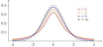
The densities of Student's distribution with degrees of freedom. As grows the tails become lighter, and as the distribution turns into the standard normal (dashed line).
The net effect of a feature is its term in the decomposition of : the product of the weight and the correlation of the feature with the target variable. The sum of the net effects equals the share of explained variance. With correlated features, however, net effects too are unstable and can even be negative; we will return to this question when we talk about the Shapley value.
Example (The bike rental forecasting problem). is a date, is the number of bikes rented; ; the standard error ; ; Intercept is the free term, the coefficient of the feature .
| Feature | Weight | SE | |
|---|---|---|---|
| (Intercept) | 2399.4 | 238.3 | 10.1 |
| season SUMMER | 899.3 | 122.3 | 7.4 |
| season FALL | 138.2 | 161.7 | 0.9 |
| season WINTER | 425.6 | 110.8 | 3.8 |
| holiday | −686.1 | 203.3 | 3.4 |
| workingday | 124.9 | 73.3 | 1.7 |
| weathersit MISTY | −379.4 | 87.6 | 4.3 |
| weathersit RAIN/SNOW/STORM | −1901.5 | 223.6 | 8.5 |
| temp | 110.7 | 7.0 | 15.7 |
| hum | −17.4 | 3.2 | 5.5 |
| windspeed | −42.5 | 6.9 | 6.2 |
| days_since_2011 | 4.9 | 0.2 | 28.5 |
UCI ML Repository: Bike Sharing Dataset. Christoph Molnar. Interpretable Machine Learning: A Guide for Making Black Box Models Explainable. 2019.
The example shows that weights and -statistics say different things. The largest weight in absolute value belongs to bad weather (rain, snow and storms reduce rentals by almost two thousand bikes a day), but the largest -statistic belongs to the feature "number of days since the beginning of 2011", whose weight is only 4.9: this feature reflects the growing popularity of the rental service and is estimated very reliably. The temperature weight of 110.7 means that each degree adds about a hundred and ten rented bikes. The season "fall" is statistically insignificant: , and the confidence interval for its weight covers zero.
Weights and -statistics describe the model as a whole. Often something else is needed: to explain why a particular forecast came out on a particular object.
Definition (Feature importance estimates for a fixed object).
- The importance of a feature (contribution, effect) :
- takes scale into account, but not shift or correlations.
- Situational importance :
- takes scale and shift into account, but not correlations.
Boxplots show the distributions , and separate marks show the effects on a particular chosen object . Such a plot explains which features produced a low forecast on the given object.
Christoph Molnar. Interpretable Machine Learning: A Guide for Making Black Box Models Explainable. 2019.
The forecast of a linear model is a sum of the contributions of the features, so the contribution is naturally taken as a measure of how much the feature influenced the answer. But the contribution is measured from zero, and zero is often nothing special for a feature: zero temperature is not the "absence" of temperature. Situational importance measures the contribution from the feature's mean over the sample and answers the question of how much this object differs from a "typical" one because of the given feature. Neither estimate takes correlations between features into account.
Visual methods: partial dependence plots
For a nonlinear model the contribution of a feature is no longer expressed by a single number. But one can draw how the model's answer depends on the feature.
Definition (Partial Dependence Plot (PDP)). How does the model depend on a part of the features ? Let , where are the features from and the remaining features.
Estimating the integral by the Monte Carlo method:
Christoph Molnar. Interpretable Machine Learning: A Guide for Making Black Box Models Explainable. 2019.
To see how the model depends on the features , the values of the remaining features are averaged out. In the first variant, the values are substituted into all the objects of the sample, and the other features are taken as they are; this estimates the integral over the marginal distribution of . The drawback is that with correlated features such substitution produces unrealistic objects — a hot day in January, for example. The second variant averages over the conditional distribution: the objects of the sample are weighted by a kernel according to how close their values are to , so that only plausible combinations enter the average. Typical plots for the bike problem: rentals grow with temperature and level off in hot weather, and fall with high humidity and strong wind.
Definition (Individual Conditional Expectation plots (ICE)). Individual Conditional Expectation is a PDP for individual objects: , where are the features from and the remaining features.
The plot of the dependence for each shows how the model's prediction on the object would change if the value of the chosen feature , , were changed.
Christoph Molnar. Interpretable Machine Learning: A Guide for Making Black Box Models Explainable. 2019.
A PDP is the mean of the ICE curves. Averaging can hide the fact that a feature acts differently on different objects: if on half the objects the forecast grows with the feature and on the other half it falls, the PDP will be almost horizontal, and the feature will seem unimportant. A set of ICE curves shows such heterogeneity at once.
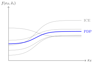
A schematic example: the ICE curves of five objects (grey) and their mean, the partial dependence plot (blue). On four objects the forecast grows with the feature , on one it falls; the PDP alone does not show this.
Interpretation in the feature space
Permutation feature importance
The next method works for any model and estimates the importance of a feature by how much the quality of the model deteriorates if that feature is "spoiled".
Definition (Permutational feature importance (PFI)).
the losses on the original sample and after shuffling:
where is the trained model, the loss function, and the object with the substitution .
Advantages: any model; training once; correlations are taken into account.
Drawback: shuffling can produce unrealistic objects.
Christoph Molnar. Interpretable Machine Learning: A Guide for Making Black Box Models Explainable. 2019.
The values of the -th feature are randomly shuffled between objects, so that the link between the feature and the answer is destroyed while its distribution stays the same. The model is not retrained: it was trained once, and on the spoiled sample only its losses are computed. If the feature matters to the model, the losses will grow noticeably; if not, they will hardly change. Since the other features are kept, the interactions of the -th feature with them also enter the estimate. The drawback is the same as with PDP: with correlated features, shuffling creates combinations of values that do not occur in the data, and the model is evaluated where it was not trained.
The Shapley value
A deeper idea came from cooperative game theory. The contribution of a feature to the quality of a model depends on which other features are in it: two strongly correlated features are each important separately, but together each adds almost nothing to the other. So a feature has to be assessed over all possible "coalitions" of features.
Definition (The Shapley value (from cooperative game theory)). The features play a cooperative game:
- is the joint payoff of a coalition , ;
- the players join one by one, in an order given by a permutation ;
- is the utility of the player in the coalition ;
- is the set of players that come before in the permutation .
The Shapley value is a fair division of the total payoff:
where is the number of ways to form the coalition ; is the number of ways to continue forming the coalition after joins ; is the number of permutations of the set of players.
Lloyd Stowell Shapley. A value for n-person games. 1952.
The meaning of the formula is this. The players enter the coalition one at a time in random order, and each is credited with what they added to the payoff at the moment of their arrival. The Shapley value is the player's mean addition over all orders. In the second form the sum runs over the coalitions that do not contain : the coalition comes before in exactly permutations.
Theorem (Shapley). The Shapley value is the only division that satisfies the axioms:
- efficiency: ;
- symmetry (anonymity of the players): ;
- no free ride for a "dummy": ;
- consistency (, are two utility functions): ;
- additivity (over sources of payoff): .
Lloyd Stowell Shapley. A value for n-person games. 1952.
The axioms are what make the division "fair". The whole payoff is distributed without remainder; players who are equally useful in any coalition get equal shares; a player who adds nothing to any coalition gets nothing; a player who is everywhere more useful in one game than in another gets no less in it; finally, if the payoff comes from several sources, the division adds up too.
Empirical estimation of the Shapley value
The exact formula requires going through all coalitions, and with hundreds of features this is impossible. But the Shapley value is an expectation over a random permutation, and it can be estimated by sampling.
Definition (Empirical estimation of the Shapley value). An unbiased Monte Carlo estimate of the Shapley value: is a random subset of permutations; for each the features , , are added to the model incrementally:
What to take as the payoff of the features :
- the coefficient of determination , with the model retrained as each feature is added;
- the Shapley regression value on the object , where the model is trained only on the features from ;
- the Shapley sampling value , where and is the mean over the sample objects : .
E. Štrumbelj, I. Kononenko. Explaining prediction models and individual predictions with feature contributions. 2014.
The choice of payoff determines what exactly is explained. If the payoff is the quality of the model , the Shapley value decomposes the quality of the model over the features: a global explanation. If the payoff is the model's answer on the object , the Shapley value decomposes that answer: an explanation of a particular prediction. The first variant needs a separate model for each coalition, trained only on its features, and that is expensive. The second variant makes do with one trained model: the absence of the features from is imitated by averaging over their values on sample objects that are similar to in the features .
The Shapley value for features in linear regression
For linear regression with the payoff , the Shapley value gives a way to correct the instability of the weights under multicollinearity.
Definition (The Shapley value for features in linear regression). is the solution of the problem .
The decomposition of the coefficient of determination into net effects:
The decomposition of into the Shapley values of the features, with :
Equating the effects, , we get .
Advantages of the Shapley estimates for linear regression:
- they are not affected by multicollinearity and are more stable;
- the coefficients are interpretable by sign and magnitude;
- they may be biased, but the bias is small.
S. Lipovetsky, M. Conklin. Analysis of regression in game theory approach. 2001.
Both sums decompose the same quantity over the features, but differently. The net effects inherit the instability of the least squares weights. The Shapley values are stable: each is the mean contribution of the feature over all coalitions, so correlated features share their common contribution between themselves instead of pulling it away from each other with opposite signs. If we require that the net effect of each feature equal its Shapley value, we obtain new regression coefficients. They no longer minimise the sum of squares exactly, that is, they have some bias, but they are stable and meaningful in sign and magnitude.
Surrogate modelling in the neighbourhood of an object
Another approach to explaining the prediction of a complex model on an object is to approximate it in the neighbourhood of by a simple interpretable model.
Definition (Surrogate modelling in the neighbourhood of an object).
-
is the training sample, the loss function;
-
is an uninterpretable model trained on the sample:
-
is an interpretable surrogate model that approximates in the neighbourhood of the object being explained:
-
are surrogate objects sampled from a radial distribution centred at with radius ;
-
are the weights of the objects in the -neighbourhood of the object ;
-
is a closeness function (kernel) of radius ;
-
is a regulariser, a penalty on the complexity of the model .
The training sample for the surrogate model is not the original objects with the teacher's answers but synthesised objects with the answers of the complex model itself. The surrogate model learns to imitate , and only in the neighbourhood of : the objects are weighted by their closeness to . The regulariser prevents the surrogate model from becoming complex, otherwise its interpretability would be lost.
The LIME method
Definition (The LIME method (Local Interpretable Model-agnostic Explanations)).
- the object for which an explanation is required is fixed;
- surrogate objects are synthesised in its neighbourhood;
- the values of the main model are computed on them;
- a local approximation by the surrogate model is built;
- an explanation and its visualisation are built for the object .
M. Ribeiro, S. Singh, C. Guestrin. "Why should I trust you?" Explaining the predictions of any classifier. 2016.
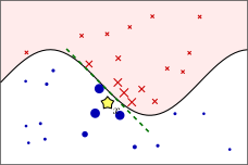
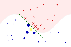
The idea of LIME (schematic): the solid curve is the class boundary of the complex model (the region of one class is shaded), the star is the object being explained. Surrogate objects are synthesised around , the size of a point being its weight ; the answers on them are given by the model . The dashed line is the linear surrogate model trained on these objects: it approximates poorly as a whole, but well near .
The method does not depend on the design of the model (it is model-agnostic): it only needs to be able to compute its answers on the synthesised objects. Globally the model can be as nonlinear as you like, but in a small neighbourhood of the object its boundary is almost straight, and a linear model approximates it well. The weights of this linear model serve as the explanation.
Definition (The LIME method: synthesising surrogate objects).
- the features ;
- synthesising a surrogate : apply to all the distortions for which ;
- synthesising a sample of surrogates : by random .
O. Sedukhin. Model interpretation and data shift diagnostics: LIME, SHAP and Shapley Flow. 2022 (in Russian).
An important detail: the features of the surrogate model are not the original features of the object but binary indicators of "distortions". The object is spoiled by a set of predefined distortions; the binary vector says which of them are applied. For example, an image of a cat is split into fragments, and a distortion is painting a fragment grey; means that the second, third and sixth fragments are painted over. The surrogate model explains the answer of on in terms of these distortions, which a person can understand.
Definition (The LIME method: interpretability of the surrogate model).
Examples of interpretable distortions of the object :
- replacing the -th feature in by a missing value, the mean value or 0;
- replacing part of the object by part of another object;
- dropping the -th word from the text , and so on.
Interpretability of the linear model :
- the weight equals the change in when the distortion is removed;
- the number must not be too large;
- there must be no multicollinearity (regularisation!).
is the quadratic loss function; , where is the Euclidean or cosine metric.
M. Ribeiro, S. Singh, C. Guestrin. "Why should I trust you?" Explaining the predictions of any classifier. 2016.
Example (LIME: text classification (20 Newsgroups)). The features ; a histogram of the weights shows the importance of the words for the original text .
The SVM-RBF classification model has 94% accuracy on test, but when distinguishing the classes "christianity" and "atheism" it considers the junk words "Posting", "Host", "Re" important. It is clear what the problem is and how to fix it (filter the words).
This example from the paper of the LIME authors shows why a developer needs explanations. By its test accuracy the model looks excellent, but the explanations reveal that it distinguishes topics by service words from the e-mail headers. In this dataset such words happen to correlate with the topic, and on new data the model will fail. Without explanations this problem cannot be seen, and once it is seen it is easy to fix: remove the headers from the texts.
Example (LIME: image classification). The features are segments (super-pixels) of the image ; , and the features are constructed for the object being explained.
The classification model is the deep neural network Inception. The three most probable classes for a photograph of a person with a guitar and a dog: "electric guitar" (), "acoustic guitar" (), "labrador" (). The explanation for the class "electric guitar" highlights the neck of the guitar: it is clear why the model confused "acoustic" with "electric".
The explanation of each class is the few image segments with the largest weights . For "labrador" the dog's face is highlighted, for "acoustic guitar" the body of the guitar, and for the erroneous "electric guitar" the neck, which really is similar in acoustic and electric guitars.
The Anchors method
Definition (The Anchors method: approximation by conjunctions).
formed by a small number of binary features or threshold conditions.
The rule tries to cover as large a region as possible of the objects that the model assigns to the same class as . It beats LIME in precision, coverage and quality of explanations.
M. Ribeiro, S. Singh, C. Guestrin. Anchors: high-precision model-agnostic explanations. 2018.
The surrogate model here is not a linear function but a logical rule, that is, a conjunction of several conditions. Such a rule is an "anchor": as long as the conditions hold, the model with high probability gives the same answer as on , however everything else changes. An example by the same authors is the sentiment analysis of two reviews: "This movie is not bad" (positive) and "This movie is not very good" (negative). LIME gives the word "not" a positive weight in the first review and a negative one in the second, and from the weights of individual words it is hard to understand how the model reasons. Anchors explain more clearly: positive, negative.
The SHAP method
The SHAP method combines both ideas: the LIME surrogate model and the Shapley value.
Definition (The SHAP method (SHapley Additive exPlanations)).
-
the features ;
-
synthesising a surrogate : apply to all the distortions for which ;
-
the increment of if the distortion is removed from the surrogate :
Three desirable properties of the local model :
- local accuracy of the approximation at the point : ;
- uselessness of a dummy, a feature missing in : ;
- consistency: as the increment grows, grows: .
Here the distortions play the role of the players of a cooperative game, and the payoff of a coalition is the model's answer on the surrogate in which the distortions from have been removed. Properties 1–3 are analogues of Shapley's axioms. The first is efficiency: on the undistorted object the surrogate model reproduces the answer exactly. It is implied here that the model's answer on a fully distorted object, , is taken as the origin; otherwise a free term is added to . The second is the "dummy" axiom, the third is consistency.
Theorem (Lundberg, Lee). The only distribution of the weights that satisfies properties 1, 2, 3 is the Shapley value:
where is the number of ones in the vector .
Theorem (The Shapley Kernel method). The Shapley value is the solution of a weighted least squares problem:
where are the weights of the surrogates:
The second theorem is remarkable in that it reduces computing the Shapley value to a weighted linear regression, that is, exactly to the LIME problem, only with special weights for the surrogates. The weights are large for vectors with very few or very many ones: surrogates in which one distortion has been removed, or only one remains, carry the most information about the contribution of an individual distortion. For and the weight becomes infinite. In practice these two surrogates do not enter the sum but act as constraints: the surrogate model must reproduce the answer of on them exactly.
Definition (The Shapley Kernel method: an implementation of SHAP).
- ⊕ The Shapley value is computed by a weighted linear regression.
- ⊕ LIME solves the same problem, but the surrogate weights are set heuristically, not optimally.
- ⊕ For large the vectors can be sampled from the distribution .
- ⊕ SHAP is better than LIME in experiments where they were compared with how experts explain the decisions of models.
- ⊖ The importance of features is estimated on unrealistic (out-of-distribution) surrogate objects.
Scott Lundberg, Su-In Lee. A unified approach to interpreting model predictions. 2017. E. Kumar, S. Venkatasubramanian, C. Scheidegger, S. A. Friedler. Problems with Shapley-value-based explanations as feature importance measures. 2020.
A drawback common to PDP, PFI, LIME and SHAP is evaluating the model on objects of a kind that does not occur in the data: the distorted surrogates lie outside the distribution on which the model was trained, and its answers on them can be arbitrary. The second paper in the list is devoted, among other things, to criticism of Shapley values as measures of feature importance.
Example (The SHAP method: an example of visualisation). The model of the probability of default is gradient boosting.
An individual explanation for a borrower : with a mean default rate of . The Shapley values are shown in colour: features with lower the risk estimate, those with raise it; the features are income, days since the last payment, the interest to be paid, the number of previous loans, age, and the number of requests to the credit bureau.
Aggregated explanations over the whole sample : on the X axis, ; on the Y axis, the features ; the colour of a point is the value of the feature ; the width of a line is proportional to the number of points.
The individual explanation shows how the estimate of 19% for the given borrower is made up from the average risk level of 6%: each feature shifts it up or down by its Shapley value. The aggregated plot is built from the Shapley values on all the objects of the sample. It shows at once both the overall importance of a feature (the horizontal spread of the points) and the direction of its influence: if the red points, large values of the feature, lie on the right, then risk grows as the feature grows.
The SAGE method
Definition (The SAGE method (Shapley Additive Global importancE)).
- SHAP: what are the contributions of the features to the prediction .
- SAGE: how the quality of the model as a whole depends on the features .
The modification SHAP → SAGE:
- : the losses are decomposed (LossSHAP);
- : the Shapley values are averaged over the sample;
- : or over a random subsample , if it takes too long.
Ian C. Covert, Scott Lundberg, Su-In Lee. Understanding Global Feature Contributions With Additive Importance Measures. 2020.
SHAP explains one prediction, SAGE the quality of the model as a whole. For this, the payoff of a coalition of features becomes not the model's answers but the negated losses of a model that knows only the features of the coalition (the others are averaged out). The Shapley values computed for each object are then averaged over the sample. The result is a global estimate of feature importance which, unlike PFI, takes their interactions over all coalitions into account.
Interpretation in the object space
The Shapley value for objects
The same cooperative game theory can be applied not to features but to training objects: how useful is each object for training the model?
Definition (The Shapley value for objects: incremental learning). Now the training objects play a cooperative game:
- is the model trained on the subsample ;
- on test objects (hold-out);
- is the utility of the training object ;
- is an unbiased Monte Carlo estimate.
Algorithm: for all ;
for all permutations , :
- ; ;
- for all :
- ; ;
- update the model by training it further on the object ;
- evaluate the model ;
- .
A. Ghorbani, J. Zou. Data Shapley: equitable valuation of data for machine learning. 2019.
The payoff of a coalition of objects is the quality of a model trained on these objects, measured on a held-out sample. The objects are added to the training sample in the order of a random permutation, and each is credited with how much the quality improved after it was added. The last line of the algorithm accumulates the mean over permutations: after permutations equals the mean of the additions of the object . Incremental learning is essential here: going through one permutation, the model is not retrained from scratch on each subsample but is trained further on the next object.
The Gradient Shapley method
The cheapest way of further training is one step of online gradient descent.
Definition (Building Shapley estimates into online gradient descent). Gradient minimisation of an additive criterion:
The incremental learning algorithm Online Gradient Descent: for all ;
for all permutations , :
- ; ; initialise ;
- for all :
- ; ;
- update the model ;
- evaluate the model ;
- .
A. Ghorbani, J. Zou. Data Shapley: equitable valuation of data for machine learning. 2019. M. Zinkevich. Online convex programming and generalized infinitesimal gradient ascent. 2003.
One pass through a permutation is one epoch of stochastic gradient descent in which the objects are presented in the order of the permutation, and the quality of the model is measured after each step. The Shapley value of an object comes almost for free, as a by-product of training, and the usefulness of an object is measured by how much its gradient step improved the model.
Interpreting objects with Shapley values
Definition (Interpreting objects with Shapley values).
- a low : outliers; such can be removed from the sample;
- a high : support, boundary objects; such are in short supply;
- a more stable estimate than leave-one-out.
Experiment (the UCI BreastCancer problem):
- removing the best objects from training, in decreasing order of ;
- removing the worst objects from training, in increasing order of ;
- adding objects similar to the best ones, in decreasing order of ;
- adding objects similar to the worst ones, in increasing order of .
A. Ghorbani, J. Zou. Data Shapley: equitable valuation of data for machine learning. 2019.
Objects with low and negative Shapley values make the model worse: these are outliers and labelling errors, and they can be removed. Objects with high values are support, boundary objects; these are exactly the objects the model lacks, and new objects similar to them are worth adding to the sample. The link with active learning is direct here. The leave-one-out estimate, the change in quality when one object is excluded, is less stable: if two objects duplicate each other, excluding either of them changes nothing, and both get a zero estimate, although together they are useful. In the authors' experiments on the breast cancer problem, removing the objects with the largest degrades quality faster than removing random ones, while removing the objects with the smallest improves quality.
Counterfactual explanations
The last type of explanation answers not the question "why did the model decide this way" but the question "what needs to change for it to decide otherwise".
Definition (The problem of finding counterfactuals). A counterfactual is an object similar to but with a substantially different model prediction .
- A credit scoring model has issued a refusal. What changes in the features would change the model's decision? (Close other loans? Move to another city? Change jobs? Change the structure of expenses?)
- A model has estimated the rental value for an owner. Which factors could increase the estimate? (Better renovation? Allow pets?)
Important: find feasible changes of the features:
- change the minimum number of features minimally;
- choose from a set of diverse counterfactuals.
Riccardo Guidotti. Counterfactual explanations and how to find them: literature review and benchmarking. 2022.
For a person who was refused a loan, the most useful thing is not a list of feature weights but advice: what they need to do to be approved. Such advice must be feasible: changing one's age or city of birth is useless, while changing the structure of one's expenses is possible. It must be economical: change as few features as possible, and as little as possible. And it is useful to offer several different options, so that the person can choose the one that suits them.
Definition (A method for finding counterfactuals (Counterfactual explanations)). A counterfactual is an object that differs minimally from and substantially in the model's prediction . In psychology, a mentally imagined alternative course of events.
The optimisation problem of finding counterfactuals with a given :
The regulariser makes the solution sparse: the larger , the more features coincide, :
Median Absolute Deviation , .
By gradually decreasing , we fit .
S. Wachter, B. Mittelstadt, C. Russell. Counterfactual explanations without opening the black box: Automated decisions and the GDPR. 2017.
The problem looks for an object on which the model gives the required answer and which differs little from . The distance is taken in the norm, and this is essential: as in LASSO, the penalty leads to a sparse solution in which most features stay unchanged and only a few change. Each feature is normalised by its median absolute deviation, a measure of spread robust to outliers, so that changes in different features are commensurable. One starts with a large , at which almost coincides with , and decreases it until the model's answer on becomes close enough to .
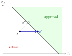
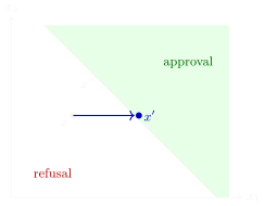
A counterfactual (schematic): the line is the model's decision boundary. The nearest point in Euclidean distance, , requires changing both features; the penalty gives a sparse counterfactual , in which one feature, , is changed and stays the same.
Approaches to the explainability of models
The taxonomy from the survey by Belle and Papantonis gives an overall picture. Interpretable models — linear and logistic regression, decision trees, nearest neighbours, logical algorithms, generalised additive and Bayesian models — explain themselves. Opaque models — random forests, SVM, multilayer neural networks — need explanations "after training" (post-hoc). Such explanations fall into several categories: simplification (replacing the model by rules or a tree), feature importance estimates (influence functions, sensitivity, game-theoretic methods), local explanations (linear approximation, counterfactuals) and visual explanations (dependence plots). Examples of methods are SHAP, Anchors, LIME, counterfactual examples, ICE, PDP, and rule extraction from tree ensembles (inTrees).
V. Belle, I. Papantonis. Principles and practice of explainable machine learning. 2020.
Summary
- Interpretability is the transparency of the model's design, or the understandability of its result on an object.
- There are not many interpretable models: linear (MVLR, LR, GAM, GLM), logical (DT, RI), metric (kNN, PW, RBF), Bayesian (NB, BN).
- Explaining a decision on an object is done, as a rule, with an interpretable surrogate model.
- The Shapley value estimates the contributions of "players" to the overall result from data on the success of their coalitions; the "players" are features, but the idea applies to objects too.
- SHAP and SAGE are the most advanced explanation methods.
P. Linardatos, V. Papastefanopoulos, S. Kotsiantis. Explainable AI: A Review of Machine Learning Interpretability Methods. 2021. Zachary C. Lipton. The Mythos of Model Interpretability. 2018. Christoph Molnar. Interpretable Machine Learning: A Guide for Making Black Box Models Explainable. 2019. Ribana Roscher et al. Explainable Machine Learning for Scientific Insights and Discoveries. 2020.
The abbreviations in the summary: MVLR, multivariate linear regression; LR, logistic regression; GAM and GLM, generalised additive and generalised linear models; DT, decision trees; RI, rule induction; kNN, nearest neighbours; PW, the Parzen window; RBF, radial basis function networks; NB, the naive Bayes classifier; BN, Bayesian networks.
No comments yet
Be the first to share your thoughts.