August 30, 2026 · Lecture · LibreTimes
Machine Learning 2. Lecture 11. Active Learning
Contents
- What this lecture is about
- The problem setting of active learning
- The active learning scheme
- The formal setting
- Why active learning is faster than passive learning
- Evaluating the quality of active learning
- Active learning strategies
- Examples of active learning applications
- Selecting objects from a sample
- Uncertainty sampling
- Query by committee
- Version space reduction
- Expected model change
- Expected error reduction
- Query synthesis (experiment design)
- Gradient-free optimisation. The Nelder–Mead method
- Variance reduction
- Density weighting
- Active learning with exploratory actions
- The need for exploratory actions
- The ε-active algorithm
- The exponentiated gradient
- Active learning in crowdsourcing
- The crowdsourcing problem
- Reconciling annotators' labels
- Models of annotator reliability
- Assigning tasks to annotators
- Summary
- Seminar
What this lecture is about
Today our topic is active learning, and it is in a sense a continuation of the previous topics. We began with forecasting methods, then looked at incremental machine learning methods, then reinforcement learning, and today active learning. What unites these four topics? That in them the objects of the training sample form a sequence, but each time we look at this in a slightly different context.
Let me start straight away by explaining the substance. The situation where the sample grows gradually and new objects appear is the problem setting we looked at last time. But here you have a huge pool of unlabelled objects, and you label them, that is, for each object you specify the correct answers . The problem is that labelling one object may cost time, money, some other resource, perhaps human, and labelling the whole sample at once is practically impossible. So one can label it gradually and train on the labelled part of the sample. But the question arises: can we somehow control which objects exactly we give for labelling, so as to label as few objects as possible, yet without harming the quality of learning?
The problem setting of active learning
The active learning scheme
The scheme is this: the machine learning model itself chooses which object from the pool of unlabelled objects to give the annotator for labelling. Then you get a labelled set, and since labelled objects arrive sequentially, you may well use incremental machine learning methods here, though perhaps there will be no need for that.
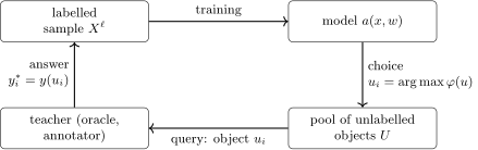
The active learning scheme: the model chooses from the pool the most promising object for labelling, the teacher labels it, and the model is trained further on one more example.
Definition (The active learning problem). The problem: training a model on a sample when obtaining the teacher's answers is expensive.
Burr Settles. Active Learning Literature Survey. 2010.
I draw your attention to a good literature survey — rather old; newer surveys are also appearing very actively, and on the last slide I will have a number of further references. So, our task is to understand by what methods unlabelled objects can be selected for labelling.
The formal setting
Let us write this a little more formally as pseudocode. We have a sample of labelled objects and a pool of unlabelled objects , and our task is to build not only a model but also to end up with a labelled subsample of objects from this pool.
Definition (The problem setting of active learning). Given:
- , a sample of labelled objects;
- , a pool of unlabelled objects.
Find:
- , a model with incremental learning;
- , a model of how promising it is to label ;
- , , a labelled sample.
Criterion: achieve the best possible quality of the model while labelling as few objects from as possible.
Algorithm:
- train the model on the initial sample ;
- while there are unlabelled objects and the model has not finished learning:
- , the most promising object;
- , request the teacher's (oracle's) answer;
- train the model further on one more example .
Burr Settles. Active Learning Literature Survey. 2010.
We start from the fact that we have some initial labelled sample, perhaps a very small one. We train the model, and then the most interesting part begins. As long as there is reason to train the model further — that is, we have a resource for labelling objects, and we consider that the model is not yet of high enough quality — we choose the next unlabelled object. The most interesting thing here is by what criterion to choose. We will need to understand what this function is, which evaluates an unlabelled object, such that by choosing objects by this criterion we learn fastest. Unfortunately, building such a criterion is an ambiguous problem: there is no unambiguously best criterion, so we will look at several. Then we label this object with the help of an annotator and train the model further; incremental learning can be applied here. The goal is to achieve the best possible quality of the trained model using as few additional examples as possible, that is, spending as little labelling resource as possible.
Why active learning is faster than passive learning
A couple of explanations of why this works after all: why we can reduce the size of the training sample in this way and improve the quality of learning.
Example (Synthetic data). Synthetic data: , ; two Gaussian classes; logistic regression on 30 objects:
- random ones;
- ones selected by the maximum classification uncertainty.
Training on a biased, non-random sample needs less data to build an algorithm of comparable quality.
Burr Settles. Active Learning Literature Survey. 2010.
Let us make a synthetic sample like this: 400 objects of two classes, two symmetric Gaussian classes. Clearly the optimal separating surface passes exactly through the middle, vertically. Let us try taking 30 labelled objects to build a classifier. The first variant: we take them at random, and the separating line comes out noticeably rotated. The second: we select them purposefully, by active learning, having chosen some criterion. Running ahead, I will say that the most obvious way of building the criterion for choosing unlabelled objects is to take objects on the boundary between the classes, on which the classification is maximally uncertain. If we select them by this principle, they are selected somewhere around the boundary and quickly build the separating surface between the classes for us — it comes out much better. From 30 non-randomly selected objects we build a better classifier than from 30 random ones. This is the first, rather direct example, an artificial one, but it explains quite clearly why active learning works.
The second example is also artificial and even simpler.
Example (A one-dimensional problem with a threshold classifier).
Let us estimate the number of steps to determine with accuracy .
- The naive strategy: choose ; the number of steps is .
- Binary search: choose the nearest to the middle of the gap between the classes, ; the number of steps is .
Let us take a one-dimensional problem with a threshold classifier: we have only one feature , say, from the uniform distribution on the interval , and the correct answers are simply the condition that is greater than zero. That is, the boundary between the classes is at zero, and our task is to discover this boundary from the training sample with such a family of threshold classifiers with parameter . Let us estimate how many steps we need to determine more or less well. The naive strategy: go through all the objects, find the two nearest ones that belong to different classes, and take, for example, the midpoint between them. The number of steps here is , in the number of unlabelled objects.
But of course we can use binary search. First let us take two arbitrary objects of two different classes — the first and the second. Then somewhere in the middle between them we find the nearest object — say, the third one. Now we have the third and the second — two objects of different classes; again we look at the middle, that is the fourth object, and so on. In this way we converge to zero quite quickly, in logarithmic time: the number of steps here is , the bisection method. This is one more illustration of the fact that learning can be arranged much faster, and far fewer objects chosen, if the right strategy for choosing objects for labelling is used.
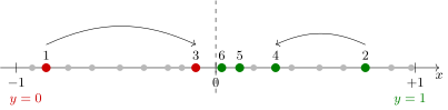
Binary search for the threshold: after objects 1 and 2 from different classes, each next object is taken nearest to the middle of the gap between the classes (3, 4, 5, 6), and the gap around the true threshold shrinks roughly by half per step. The grey points are unlabelled objects of the pool.
Evaluating the quality of active learning
Definition (The learning curve). The learning curve is the dependence of the classification accuracy on test on the number of labelled objects .
Burr Settles. Active Learning Literature Survey. 2010.
This is how the quality of active learning is usually evaluated: a learning curve is built. The figure compares two strategies. The first is when we choose objects for labelling purely at random, random; the second is sampling unlabelled objects by some criterion, for example by classification uncertainty; we will look at the criteria in a moment. The main thing is that the curve for the second strategy goes faster, higher. Perhaps it also reaches a higher level of the horizontal asymptote, but that is not at all necessarily so. At least we expect it to grow faster: such a strategy gathers a training sample more economically and faster.
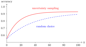
The learning curves of two strategies (schematic): test accuracy as a function of the number of labelled objects . Uncertainty sampling gains quality faster than random choice of objects.
Active learning strategies
What active learning strategies are there in general?
Definition (Active learning strategies).
- Selecting objects from a sample (pool-based sampling): which next to choose from the pool .
- Synthesising objects (query synthesis): at each step synthesise an optimal object .
- Selecting objects from a stream (selective sampling): for each arriving , decide whether it is worth learning .
Cost-sensitive methods:
where is the cost of losses for the model , is the cost of obtaining the label , is a subset of objects to be labelled.
The problem we are now discussing is selecting objects from a sample of unlabelled ones, that is, there is a large pool of unlabelled objects in advance. This situation is somewhat similar to semi-supervised learning: a small number of labelled objects and a huge number of unlabelled objects known in advance. We know them all, and so we can choose among them.
There is a completely different situation, where objects have to be synthesised. We do not have a finite set of unlabelled objects, but we can obtain the next point in the object space, as it were assign an object. This is also called experiment design. Such experiments are very often needed in industry, in particular in chemistry: what set of parameters of the technological process must be set for the next experiment to get the most successful result? This is what is called experiment design, or query synthesis in active learning terms.
There is one more problem that we will not look at today, but it is close to the first: when there is a stream of objects and we must decide about each arriving object whether it is worth labelling or not. In principle the problem setting is similar to the first, so we will not pay attention to it today.
And, in solving a machine learning problem, we can in principle take into account how much it costs to learn on the next object. One can even say that if the problem is posed strictly as an optimisation problem, we want not only to get maximum quality in training but also to reduce the cost of our losses associated with forming the labelled dataset. Such criteria are called cost-sensitive. One can build into them literally the costs in roubles or dollars, that is, compare the price of an error with the price of obtaining a labelled object: if we can measure both in money, we can write out a single criterion altogether. This approach too is sometimes used in practice, but today we will hardly touch on it, and will mainly deal with pool-based sampling and a little with query synthesis.
Examples of active learning applications
Example (Examples of active learning applications).
- collecting assessor data for information retrieval, analysis of texts, signals, speech, images, video;
- including on crowdsourcing platforms;
- experiment design in the natural sciences or in production (an example is combinatorial chemistry);
- optimising functions that are hard to compute (an example is hyperparameter optimisation, AutoML).
Business applications:
- managing prices and the product range in retail chains;
- choosing goods for a marketing promotion;
- proactive interaction with customers;
- selective quality control;
- detecting anomalies in data, cases of fraud.
Let us talk a little more about where this is applied. There are a huge number of applications. In information retrieval, these are first of all the problems of ranking search results; analysis of texts, signals, speech, images — when you need to label, say, music tracks, or some texts, or images, and you want to build a classifier on them and of course want to minimise the labelling costs. Crowdsourcing platforms are usually used for this; at the end of the lecture we will talk in a little more detail about how crowdsourcing is arranged and how active learning in particular is applied to it.
I have already spoken about experiment design. The clearest example is probably combinatorial chemistry, which is used in particular to search for catalysts. In chemistry there is still no general theory of catalysis, but there are a huge number of experiments in which a catalyst is synthesised, then a chemical reaction is carried out, and both may be an expensive and lengthy process. What should the technology for making the catalyst be? A whole range of parameters of the technological process has to be set, and all these parameters are combined all the time, in order to run as few experiments as possible and find a successful catalyst as quickly as possible. In such experiments this is a rather typical situation: we need not to choose a point from a pool of unlabelled ones but to synthesise the next point in the space of experiment parameters, and to find it as efficiently as possible.
This should be familiar to you from how you usually optimise hyperparameters in machine learning problems. With the parameters that are trained on the sample everything is clear: an optimisation problem is solved. But usually there are also some exogenous parameters — the number of layers of a neural network, the number of neurons in each layer — that have to be searched over, and the question of how to choose these parameters is also a question of experiment design. The space of hyperparameters is usually a difficulty in that it is large: if there are already ten parameters, you always face the problem of how to set up the experiment properly so as to find a decent combination of hyperparameters in this space quickly. If there are one or two hyperparameters, you usually optimise over a grid, but if there are already ten, some smarter methods have to be applied here, and I will tell you a couple of such methods today.
The business applications are clear too. For example, managing prices and the product range in retail chains is also an active experiment. You are, for example, looking for how you can lower a price a little so as to raise the demand for some product a lot. You do not want to lower it much, so as not to go into the red, but you also want to probe this dependence of demand on price — with as few erroneous experiments as possible.
Selecting objects from a sample
Now we will go into mathematics and look at different constructions of the function .
Uncertainty sampling
The very first and simplest thing that comes to mind, and in fact often used in practice, is uncertainty sampling. Today we will mainly consider the multiclass classification problem, because most often the problem of human labelling, when an annotator labels something, is precisely a classification problem, and as a rule a multiclass one: the annotator gives some ratings or does some tagging. This problem is simple for a person. It is harder to think of a situation where some numerical estimate would be required of a person; classification, as a decision-making task, is simple and more understandable to people. So, based on practice, today we will mainly look at the multiclass classification problem.
Definition (Uncertainty sampling). The idea: choose the with the greatest uncertainty of .
The multiclass classification problem:
, , are the , , ranked in decreasing order.
The least confidence principle:
The minimum margin principle:
The maximum entropy principle:
Suppose our classification model is arranged as follows: for each class an estimate of the posterior probability of the class on the object is built. For each unlabelled object you can compute such a discrete distribution over the classes with the model, and the classifier simply assigns the object to the class that seems most probable to it. Let us take these probabilities and rank them in decreasing order.
What is uncertainty sampling? It can be done in different ways. The first is the least confidence principle. You have ranked all the probabilities on the object in decreasing order and look at the first. If it is large, this means your classifier confidently assigns the object to one of the classes. The smaller it is, the more the distribution resembles the uniform one: the very minimum is attained precisely on the uniform distribution. So we can choose the object on which is minimal.
But it does not have to be done exactly so. Look at when else we have great uncertainty: when the first and second probabilities in ranking order are similar to each other. It is not necessary for the whole distribution to be uniform; it is enough for the first two probabilities to be similar, and then you will already have an uncertain classification. So another principle is the minimum margin principle, . If this difference is small — and if it equals zero, you simply have equal probability estimates for the two most probable classes — you are in a state of uncertainty.
And finally, one can use the entropy criterion, the maximum entropy: simply evaluate the whole distribution at once, estimate the entropy of the distribution, and again its maximum will be attained on the uniform distribution.
Remark (Three uncertainty criteria). In the case of two classes these three principles are equivalent. In the case of many classes differences appear.
Example. Three classes, . The level lines of the three object selection criteria on the simplex: , , .
Burr Settles. Active Learning Literature Survey. 2010.
If we look at how these criteria are arranged, in the case of two classes they are in fact equivalent to each other: they will always choose the same object. For three classes this is no longer so. The slide shows how the level lines of these three criteria are arranged on the simplex in three-dimensional space, and one can see that they are different: for least confidence the level lines are hexagons around the centre, for minimum margin the region of uncertainty is stretched along the three segments where the two highest probabilities coincide, for entropy the level lines are smooth curves. Which of them is better cannot be said: in one problem one may work a little better, in another another. This depends very much on how many classes there are and how frequent they are; there can be many different reasons. In general, one can try all three.
Remark (Why least confidence). What is the least confidence principle? You took the probabilities of the classes on an unlabelled object and ordered them in decreasing order. In which case is minimal? When this distribution is uniform, that is, when all equal . For us the maximally uncertain object is the one on which the largest probability is the smallest: the largest probability of a class is small, and the smaller it is, the more uncertain our classification, the more smeared the distribution over . The centre of these figures on the simplex is exactly the uniform distribution, and for all three criteria it is the most advantageous one for taking this object for labelling. But if you have no object in the centre, these criteria simply evaluate objects somewhere in the middle differently: these criteria are arranged a little differently, but all of them prefer to choose objects from the centre, where all the probabilities are equal.
Now we will gradually complicate this simple idea, uncertainty sampling, because this simple principle does have certain drawbacks.
Query by committee
The first complication: let us, as in ensembles, build not one classification model but several — a committee of models. If we have not one model but many, then probably our decision about which object we are more uncertain on will be more correct, more balanced. As before, each model gives a probabilistic estimate, that is, each model has its own probability distribution on the set of classes.
Definition (Query by committee). The idea: choose the with the greatest disagreement among the decisions of a committee of models
The maximum entropy principle: we choose the on which the differ most:
The maximum mean KL divergence principle: we choose the on which the differ most:
is the consensus of the committee.
The maximum entropy principle: let us choose an object on which the classifications of the models differ most. How can the difference be measured? For example, we introduce an averaged distribution — simply a frequency estimate of the class obtained by averaging over all the models. What is the drawback? That the models originally gave probabilistic estimates, and here we coarsened them with a threshold rule, with , and computed the mean. This estimate will be quite reliable if is large, but if is small, it is a great pity that we have lost the information about the distributions here.
How not to lose it? Hence the next principle, the maximum mean KL divergence principle, which relies on averaging the probability distributions themselves over the whole committee. A probability distribution is built that is a mixture of the distributions of all the models; let us call it the consensus. And we look at which object the distributions of the models will differ most from the consensus. That is, we choose the maximally uncertain object, on which the committee of models strongly disagrees, so to speak. The idea is that we build many different models, each having its own view of where its boundary between the classes lies, and so on average we will choose the object more correctly.
Version space reduction
But that is not all yet; let us see what other heuristics there are.
Definition (Version space reduction). The idea: choose so as to narrow the set of solutions as much as possible.
Boosting and bagging find finite subsets of solutions. So query by committee is an approximation of the version space reduction principle.
Let us choose an unlabelled object such that it narrows the set of solutions as much as possible. What does this mean? Suppose we have labelled objects of two classes, and suppose we use linear classifiers. A linear separating surface can pass in different ways. Clearly, to reduce this set of admissible classifiers as much as possible, we need to choose a point somewhere in the middle and get its classification; then this set will shrink roughly by half. And so each time we will shrink it roughly by half — recall the example with bisecting an interval; here it is simply a more complex situation. This is an attempt to say, for an arbitrary family of separating surfaces, that out of the whole set of admissible separating surfaces we must, by choosing the next point, reduce it as much as possible.
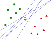
The space of admissible solutions (schematic): all the lines separating the labelled objects of the two classes are consistent with the sample. An object in the middle of the gap splits these lines: whatever answer the teacher gives on it, about half of the admissible solutions will drop out.
In a sense this is similar to what happens in boosting and bagging: there too we find a finite subset of solutions and then average them somehow. Something similar can happen here, only instead of averaging we try to reduce this set of admissible separating surfaces as quickly as possible. And query by committee is also in a sense an approximation of this version space reduction principle.
Expected model change
But that is not all yet. Let us imagine that we use some method based on stochastic gradient descent — say, we build a neural network. The idea: the most uncertain object is the object on which our gradient step would be the largest. That is, the object which, if we chose it in the stochastic gradient method, would give us a gradient step of the largest size: the norm of the gradient would be maximal.
Definition (Expected model change). The idea: choose the that would lead to the largest change of the model in the stochastic gradient method.
A parametric multiclass classification model:
For each and we estimate the length of the gradient step in the parameter space when the model is trained further on ; let be the gradient vector of the loss function.
The maximum expected gradient length principle:
Where is the catch? That in a classification problem the gradient can be computed only if you already know on this object. And we are about to choose an unlabelled object, for which we do not know . How to get round this? We have a parametric multiclass classification model and an estimate of the posterior probability . So we can estimate not simply the length of the gradient step but the expectation of the length of the gradient step over this probability distribution. Hence the maximum expected gradient length principle. We take the gradient of our loss function on the object with the answer ; we do not know the answer on this object, so we take all answers with the probabilities given by our probabilistic classification model, and take the object whose expected gradient length is maximal.
Remark (Why the expected gradient length). Which object is the most useful to us? Remember, when we talked about neural networks, we discussed that if the loss function has horizontal asymptotes, so-called network paralysis arises: we get into a point where the value of the gradient is close to zero and cannot get out of it in any way. What are these points? As a rule, they are objects that are classified well: there the derivative of the loss function is close to zero, there is the horizontal asymptote where the penalties no longer change. This suggests to us that there are situations where taking a gradient step is useless: it is very small. If an object is classified so well, there is no point in spending time on a gradient step on this object. Boundary objects, on the other hand, are in the most active region of the loss function: there the gradient is maximal, the derivative of the loss function is large there. That is, it makes sense for us to choose objects that will give us the largest gradient step.
This is simply another view of where the boundary objects lie. From the point of view of gradient optimisation, of stochastic gradient, boundary objects are those on which we get the largest further training of the model, on which the gradient step is largest. Hence the idea of choosing an object by the maximum gradient step. But the problem is that the gradient step depends on , which we do not know on this object. That is why we make an estimate by the expectation: our model assumes what there may be on this object , and for each we can compute the gradient step. If on average over all the gradient step comes out large, that is, whatever class we assign it to we will have a large gradient step, that is exactly a boundary object.
Expected error reduction
But that is not all yet. Let us realise that in fact we would like to choose an object that would be maximally useful to the classifier. What does maximally useful mean? On the one hand, it modifies our classifier as much as possible, further training on this object changes our model as much as possible; the previous principles are exactly of this kind, we have already tried them. But we want not just any change, but a change that would improve generalisation ability: the learning curve must grow as fast as possible, and it measures precisely generalisation ability, since it is computed on test data. How could we estimate the improvement in the classifier's generalisation ability if we add one more object to the training sample? This is the principle that really interests us. It is of course complex; we will now try to implement it; we have arrived at it gradually, complicating the construction of the criterion .
Definition (Expected error reduction). The idea: choose the that after further training will give the most confident classification of the unlabelled sample .
For each and we train a classification model by adding the example to the labelled training sample :
The principle of maximum confidence on unlabelled data:
The principle of minimum entropy of unlabelled data:
The idea: we choose an object that after further training will give the most confident classification of the whole unlabelled sample without this very object. Clearly, if the sample is very large, some part of it can be sampled at random, but these are details; suppose we evaluate on all the unlabelled objects. For each unlabelled object and each class we build a classification model that is trained on the current labelled training sample with the example added to it. That is, we must go through all the unlabelled objects and try for each: what if we assign it to class ? And for each such pair we train a probabilistic multiclass classification model.
Clearly this has to be incremental learning. We have a labelled training sample, we add one object to it, get a classifier, remember it, then throw this object out, add another to the training sample — all this is incremental addition of one object at a time, and each unlabelled object has to be added in this way. We build a huge number of classifiers: their number equals the cardinality of the set multiplied by the cardinality of the set . But since this is incremental further training, let us hope that we will train a classifier rather quickly. And if our set is too large, we will sample objects from it somehow at random or by a simpler method. In the end we get a pile of probabilistic classification models indexed by the pair .
And what do we want to do now? Here too several constructions arise: generalisation ability can be estimated a little differently. For example, the principle of maximum confidence on unlabelled data. We look for an object that maximises this construction: the expectation over all classes for the unlabelled object , that is, the expected estimate, and under it the confidence of classifying the unlabelled object with the model . That is, we want the unlabelled objects to be classified as confidently as possible. This is a little the other way round: before, we chose an object on which the classification was uncertain, and now we choose an object after adding which to the training sample all the other unlabelled objects are classified as confidently as possible. Such is the play on confidence and uncertainty.
And just as we began with uncertainty, confidence can be estimated by the maximum probability, or by entropy: one can introduce the criterion of minimum entropy of unlabelled data.
But this method is already outer space, and it is actually good to combine it with some simpler methods. With a simpler method you, for example, select a small number of objects , and with this more sophisticated and subtler method you can choose among these objects the one that is most advantageous from the point of view of improving generalisation ability, that is, from the point of view of the fastest growth of the learning curve.
Query synthesis (experiment design)
We have looked at a pile of methods for selecting objects from a pool of unlabelled objects, what is called pool-based sampling. Now let us look at methods that synthesise objects — that is, experiment design.
Gradient-free optimisation. The Nelder–Mead method
Here I want to tell you about one very old method, the Nelder–Mead method, which has still not lost its relevance. It is still often used in practice, partly because there are ready implementations of this method in abundance, and they have long been well debugged and work well. And even though no complete convergence theory has yet been built for this method, and even some sophisticated counterexamples have been given on which this method does not converge, nevertheless in practice it works rather fast, is easy to implement, and is still actively used.
Definition (Gradient-free optimisation. The Nelder–Mead method). The idea: choose the objects not from a finite pool but from the whole of , maximising by any gradient-free method.
The Nelder–Mead method: moving and deforming a simplex of points in the space of dimension .
J. A. Nelder, R. Mead. A simplex method for function minimization. 1965.
So, we solve the problem of maximising some criterion , and this criterion is hard to compute, and we assume that we cannot compute its derivatives. That is, we must use gradient-free methods — optimisation methods that compute the next point only from the values of this functional at some points.
The idea of the method: we build a simplex of points in a space of dimension . If our objects are vectors in a space of dimension , then to estimate the direction in which the criterion increases we will use points; this is a simplex. In two-dimensional space, , a simplex consists of three points, it is a triangle. And we will roll this triangle and perhaps deform it somehow, so that in the end it moves in the direction where the value of the criterion increases; at the same time the triangle must contract, shrink in size. A simplex in general is a way of estimating from points the direction of the maximum increase of the criterion. It is a kind of surrogate for the gradient method: we cannot estimate the gradient, but we can approximately estimate the direction of the maximum increase of the function, knowing its values at the vertices of the simplex. Starting from some triangle, we roll it over its edges, it gradually deforms and as a result contracts to a point that is close to the optimum.
How does this happen? Take the worst point of the points of the simplex — worst. The direction from this point through the middle of the opposite face of the simplex is the direction in which our functional increases. Clearly this is not an ideal direction, but, sorry, we cannot compute the gradient. Then we can compute the value, for example, at the reflected point, reflected: in the two-dimensional case it completes the triangle to a parallelogram. Let us see whether the value has improved much there. If it has improved much, let us try going even further and improving even more: there is the option of taking the point expanded, going even further — this is a kind of analogue of choosing the size of the gradient step. If nothing much worked out with reflection and expansion, we will try, on the contrary, to contract this triangle, reduce its size: we take a point inside the triangle. In principle we go through these three points, but we go through them carefully, so that we do not always have to compute all three at once: we remember that computing is expensive. So there will be a whole construction of ifs that tries these three alternatives in a certain order. And if they all turned out not very good, it remains for us to contract the triangle as a whole: the two worst points — worst and other, the second from the end — we pull towards the best. This is the situation when we are already close to the optimum: we did not manage to move away from this triangle successfully in any direction, and did not even manage to contract it along one direction; then we contract it along two directions at once. Such is the heuristic.
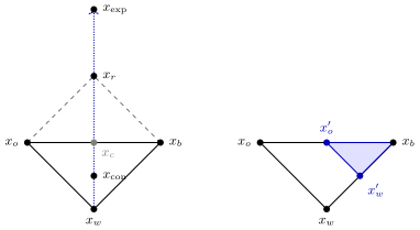
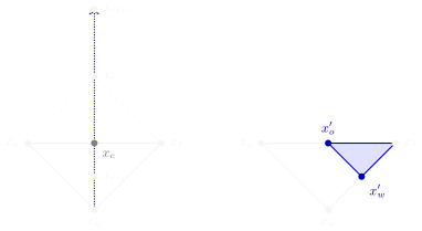
The Nelder–Mead method on the plane. Left: the worst point is reflected through the centroid of the opposite face into ; on success an expansion to is tried, on failure a contraction inwards to . Right: if nothing helped, the whole simplex shrinks by half towards the best point .
Definition (The Nelder–Mead method: "reflection–expansion–contraction"). repeat
- sort the points: ;
- the centroid of the face , over all points except ;
- reflection: ;
- if , then
- expansion: ;
- if , otherwise ;
- else if , then ;
- else
- contraction: ;
- if , then ;
- else shrink the simplex: for all ;
until .
Recommended parameters: , , , .
This pseudocode is given in many textbooks on optimisation; here the same idea is simply set out more carefully. We order all the points of the simplex: from the word worst, from the word other, the second to last, from the word best, the best point. Then we find the centroid and do the reflection — compute the reflected point . If all went well and is better than best, we try expansion: the triangle rolls over its edge, and we try to go even further. If the reflected point is worse than the best one, we need not go further in this direction. If it is at least better than , we simply replace the worst point with it; and if not, we stay inside the triangle and try to compute the contracted point , and if it too is not good enough, we shrink the whole simplex towards the best point.
This method has parameters that say where the reflection should be taken: usually , which means a symmetric reflection, that very parallelogram; there are also the parameters , and . These parameters say how you should choose the next points from this triangle. There are recommended values; one can try to tune them, but this usually affects little.
Such is this rather neat method, with which for more than half a century people have been doing experiment design in the most varied applied fields. And I say again what is close to us: in data science we very often do non-trivial hyperparameter selection in some low-dimensional space, and for this the Nelder–Mead method is quite good, because it works much faster than grid search or random search. In general, please welcome it.
Variance reduction
One more situation, a little different: here we will talk about solving a regression problem, and as the measure of uncertainty let us take the variance. If we train the model further on some object, what variance will the regression model have? This is one more criterion by which a new object can be chosen.
Definition (Variance reduction). The idea: choose the that will give the smallest variance estimate after the model is trained further on .
The least squares method, linear regression :
From the theory of optimal experiment design (OED):
The variance reduction principle for linear regression:
Burr Settles. Active Learning. Morgan & Claypool Publ., 2012.
Since we are in a linear vector space, the problem here is to choose not from a pool, a finite set of objects, but simply an arbitrary point in the linear vector space that will give the smallest variance estimate . We solve a regression problem by least squares, that is, we choose the parameter of the regression model, and is the so-called residual sum of squares.
There is a whole theory of optimal experiment design in which such an estimate is proved, and in a rather general form, for an arbitrary model — including a nonlinear one, but smooth in the parameter . If we take an arbitrary point at which we compute our model, already trained on this training sample by least squares, we can estimate the variance at it — how large a spread of values, purely random, there can be at this point. The formula requires knowing the partial derivatives with respect to the parameters for the model itself and for the residual sum of squares. This expression looks rather cumbersome, but clearly in each particular case, for a particular form of model, it can easily be computed. For linear regression it is an expression we already know: the matrix , inverted. We have already seen it in multivariate linear regression problems and understand that it can be computed by SVD. This thing inevitably arises in solving the least squares problem for linear models and if one uses second-order stochastic gradient methods. So in many methods we simply have it at hand, and it can be used to compute variances.
In this way we construct a criterion that lets us choose a point. This criterion can be used both to choose a point from a finite set of unlabelled objects, from a pool, and to solve the optimisation problem of synthesising a point with the largest variance. The largest variance is simply, for a regression problem, a more correct principle of maximum uncertainty: until now we dealt with classification problems and expressed uncertainty through the conditional probability distribution over the classes, while here maximum uncertainty is on the objects where the variance is maximal. And there is a variance estimate that comes from the theory of the least squares method.
Density weighting
We have practically finished with the criteria, and now let us look at one more problem that arises in practically all problems, regardless of which criterion we use — the problem of unrepresentative objects.
Definition (Density weighting (density-weighted methods)). The idea: lower the weight of unrepresentative objects.
Any object selection criterion of the form
can be refined by a local density estimate:
where is an estimate of the closeness of and (the closer, the larger).
Imagine this picture: the labelled objects are coloured, the white dots are unlabelled, and you choose the most boundary object by some uncertainty criterion. And you end up choosing the object . From the picture it is clear that this is an unrepresentative object, and adding it to the training sample is on the whole not very good: it is rather a noise outlier. In this case choosing the object would be preferable. But a pure criterion of uncertainty, or of how boundary an object is, will not let you choose in this situation.
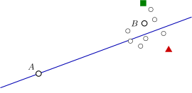
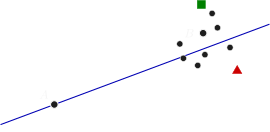
An unrepresentative object (schematic): the line is the current separating boundary, the white points are unlabelled objects. The object lies right on the boundary but far from the rest; the object is a little less on the boundary, but is surrounded by other unlabelled objects. Density weighting will prefer .
Let us correct the criterion somehow to take the representativeness of an object into account, that is, multiply by some factor that will depend on how densely the objects are located around our object : the denser, the better, and the more likely we are to choose this object. How can this be done? For example, sum the closeness measures over some neighbourhood of the object ; it can be raised to a power; in general one need not limit oneself to a multiplicative criterion and can arrange an additive one — this is on the whole not very important; many different heuristics can be devised here. And which estimate of the closeness of objects in the object space to use I do not write here either, since it depends on each problem. The main idea is that we can multiply the object selection criterion by some estimate of the representativeness of this object, such that it is the larger, the higher the local density of objects in its neighbourhood. Such is one more rather important heuristic, density weighting.
Active learning with exploratory actions
The need for exploratory actions
Now we will look at one more important aspect of active learning, which in a certain sense brings active learning and reinforcement learning closer together. In active learning, exploratory actions are also very important, that is, the exploration–exploitation balance, which in reinforcement learning is almost a cornerstone.
Definition (The need for exploratory actions in active learning). Drawbacks of active learning strategies:
- regions of the space remain unexplored;
- as a result the quality of learning decreases;
- the training time increases.
Ideas for using exploratory actions (similar to exploration/exploitation in reinforcement learning):
- take a random object with probability ;
- adapt the parameter , decreasing it over time, depending on the success of the exploratory actions;
- reinforcement learning can be used.
D. Bouneffouf. Exponentiated gradient exploration for active learning. 2016. D. Bouneffouf et al. Contextual bandit for active learning: active Thompson sampling. 2014.
Here too it is important to choose some random object from time to time, otherwise some regions of the space may turn out not to be evaluated at all. From the model's point of view an object may be evaluated as confident, not boundary, but it may turn out that it is important for further training after all. How not to miss such objects? Otherwise the classifier may be built only for some part of the sample, and a very important part of the sample may turn out to be unexplored altogether.
What could the idea be here? On the whole, the same as in ε-greedy algorithms for reinforcement learning: let us take a random object with some probability. Probably this probability should be gradually decreased over time. And can the parameter be adapted depending on how successful the exploratory actions were?
Whether exploratory actions are needed or not depends in fact on such a tricky point as how correct the model chosen for the given problem is. If you have chosen the model well and in principle it describes the boundary between the classes quite well, you do not really need exploratory actions. But if the model does not describe the boundary between the classes very well, a nuance arises here, and perhaps you need such randomly chosen objects from some distant parts of the object space.
The ε-active algorithm
This method is called ε-active, and in fact it differs little from what we have looked at so far. From the very beginning this is our main pseudocode, and what is added is this: now with probability we choose any unlabelled object purely at random, from the uniform distribution on our pool of objects, and with probability we act as before, that is, we maximise the criterion . Such is a small addition to the algorithm we had at the very beginning.
Definition (The ε-active algorithm). The algorithm is a wrapper over any active learning strategy.
Input: the labelled sample and the pool .
Output: the model and the labelled sample .
- train the model on the initial sample ;
- while there are unlabelled objects and the model has not finished learning:
- choose : with probability , a random unlabelled one (from the uniform distribution on ); with probability , ;
- learn for the object ;
- train the model further on one more example .
The problem: how to choose the probability of exploratory actions? How to adapt (decrease) it over time?
The exponentiated gradient
Can this probability of exploratory actions be chosen based on the actual need for such actions? Here a method called the exponentiated gradient comes to the rescue. In general the exponentiated gradient appears in machine learning in different contexts: it can be used to build compositions, ensembles, and, say, in the problem of optimal investment portfolio choice, portfolio selection — we mentioned this problem once — this method is also actively used. That is, it is rather universal.
Definition (The exponentiated gradient (Exponential Gradient)).
- is a grid of values of the parameter ;
- are the probabilities of using the values ;
- , , are parameters of the method.
The idea of the EG-active algorithm: as in the AdaBoost algorithm, increase exponentially in case of success of :
- exponential update of the weights by the value of the criterion on the chosen object :
- renormalisation of the probabilities:
D. Bouneffouf. Exponentiated gradient exploration for active learning. 2016.
It is used here as follows. We introduce a grid of values of the parameter and the probabilities with which we will use these parameter values. This is also somewhat reminiscent of evolutionary algorithms of the stochastic adaptive search type. Then we will increase these probabilities if using the given value of the parameter led to success. How to measure success? With this heuristic: we are always looking for an object that maximises for us, and if turned out large, that is our success. Then we use a transformation with the parameters and and compute the weight coefficient , which is the larger, the more successful our parameter was. Then we simply normalise these weight coefficients and convert them into the probabilities . This construction resembles softmax, except that there is also a probabilistic mixture with the uniform distribution, just in case, with some factor : a convex combination of our normalised probability distribution and the uniform distribution, so that all the still keep some non-zero probabilities and all have a chance of being chosen.
This is a technique that can in fact be applied not only here; take note. Again, the same hyperparameter optimisation over a grid of values. We can choose a value on the grid several times and understand where the working zone is on this grid, where the values are that are better taken with greater probability. If we make sampling over the grid probabilistic, this lets us find the optimum faster than a simple exhaustive search over the grid. It is a more efficient scheme of probabilistic search over grids with adaptation of the probability distribution on the grid of values. The exponentiated gradient is exponential because such a multiplicative formula is used for updating the weights by the values of the criterion: the more successful a grid node, the larger its probability will be. But generally speaking, it is a heuristic: has to be computed so that it increases as the obtained with the given grid value increases, and this can be done in different ways, not only as proposed here — other heuristics can be devised.
Definition (The EG-active algorithm). Input: , , parameters , , , .
Output: the model and the labelled sample .
- initialisation: , ;
- train the model on the initial sample ;
- while there are unlabelled objects and the model has not finished learning:
- choose from the discrete distribution ;
- choose : with probability , a random unlabelled one; with probability , ;
- learn for the object ;
- train the model further on one more example ;
- ;
- for all .
D. Bouneffouf. Exponentiated gradient exploration for active learning. 2016.
How does this algorithm differ from what we had before? The new elements are elements of the ε-greedy strategy: we use the parameter as the probability with which we choose a random unlabelled object. And depending on how successful the choice of this unlabelled object turned out to be, we adapt the probability distribution on the grid. So we have seen how exploratory actions can be inserted into active learning: the simple ε-active algorithm and a more advanced algorithm that adapts the grid of values of probabilistically.
Active learning in crowdsourcing
The crowdsourcing problem
Now one more topic of interest, quite different — crowdsourcing. Crowdsourcing is a special case of active learning. It differs in this. If we go back to the very beginning, to the original scheme, we have one annotator sitting there — a clever one who gives correct answers on the objects . But the trouble is that nobody has cancelled the human factor: even if the annotator is clever, they can sometimes make mistakes; they are only human. And if there are many annotators and they are cheap, they will most likely make mistakes often, and we compensate for the annotators' insufficient competence by their number. That is crowdsourcing.
Definition (Active learning when there are many annotators). are the answers of the annotators on the object .
The problem: form an agreed answer (consensus) and estimate the reliability of each annotator .
R. A. Gilyazev, D. Yu. Turdakov. Active learning and crowdsourcing: a survey of data labelling optimisation methods. 2018 (in Russian).
And now a whole pile of questions arises. The first problem we know how to solve: we choose an unlabelled object. But we send it not to one annotator but to a whole bunch of annotators, and each annotator gives their own answer on this object. Naturally they may contradict each other; some of them make mistakes. The first problem that arises here is to estimate the reliability of an annotator. At first sight it can be solved rather easily: if there are many annotators, let us choose some agreed answer, for example the one the annotators give most often, some average answer. Then the reliability of an annotator can be estimated by how often their answers agree with this correct answer, with the consensus of the annotators.
But that is not the only problem. There is another problem: can we choose an annotator who is more likely to label the given unlabelled object correctly? We naturally want to save resources and to understand as quickly as possible on which objects each annotator gives more correct results. Each annotator may have their own area of competence, they may have their own biases, that is, in some situations they will make systematic errors. How to choose the annotators who will label the given object most correctly? This is one more problem. Let us look at this whole complex of problems gradually. By the way, there is a good survey made at the Institute for System Programming, rather recent and in Russian: if anyone needs to get to grips with active learning and crowdsourcing, look there.
Reconciling annotators' labels
Definition (Reconciling annotators' labels).
- is the answer of the annotator on the object ;
- is the set of annotators who labelled the object .
The consensus is a weighted vote of the annotators:
is the weight of the annotator in the vote, for example:
- for majority voting (MV);
- under the assumption that the annotators are independent.
An EM-like algorithm for reconciling the annotations of the object :
until the estimates converge:
- estimate the consensus ;
- estimate the reliabilities and the weights of the annotators;
- if , exclude the annotator from the estimate.
So, we have the answers of different annotators on one and the same unlabelled object, and let us denote by the set of annotators who labelled the given object; the question of how we chose this set of annotators we leave aside for now — suppose it has been chosen somehow. A weighted vote of the annotators is simply a generalisation of the estimates I have just written: we get as a result of averaging the annotators, but we want to take each annotator into account with a weight.
And the question arises: how to estimate the reliability of the annotators, their weight in the vote? The simplest way is just to set the weights equal to one; this is if we know nothing a priori about which annotators are better and which are worse. A smarter way is to use the naive Bayes classifier. Annotators are in fact something like features for us, and a weighted vote is in effect a linear classifier. If we assume the features are independent, that is, the annotators are independent, there is an analytical expression for the weight coefficient: the logarithm of the ratio of to , where is the reliability of the annotator, an estimate of the probability that they give the correct, that is, the agreed, answer . The larger , the higher the weight of the annotator. The more often an annotator gives the same answer as the majority, the more reliable they are: they agree with the majority, they are adequate, and is in a sense an estimate of the annotator's adequacy. Of course, the independence of the annotators is a rather strong assumption. Annotators will of course not be independent, if only because in serious crowdsourcing problems annotators usually go through some training, they are given the same instructions, they try to follow the same rules. Nevertheless it is still a better estimate than just one.
Here we can use an algorithm that is similar to the EM algorithm, and perhaps even somewhat to the -means clustering algorithm. It is based on this two-step procedure: it is an iterative process, at each step of which we first estimate the correct answer by this formula, given that we have the annotators' weights initialised somehow, for example uniformly; then we estimate the reliabilities — the share of objects that the given annotator rated the same as the majority — and recompute the annotators' weights from them. And we do this until the estimates and converge. Then we have reconciled the annotators with each other and determined their weights. There are many varieties of such an algorithm, but the general idea is to reconcile the average estimate and the estimates of the annotators' reliability .
Models of annotator reliability
In fact the reliability of annotators can be modelled in different ways, and there are many different approaches.
Definition (Variants of modelling annotator reliability).
-
From the results of test tasks.
-
Modelling the confusion matrix :
-
Modelling the difficulty of objects:
is a frequency estimate of the reliability of the annotator ; is an estimate of the difficulty of the object (for a large ).
-
Modelling the topical competence of annotators: is a topical vector representation of the object , for example if the object is a text.
R. A. Gilyazev, D. Yu. Turdakov. Active learning and crowdsourcing: a survey of data labelling optimisation methods. 2018 (in Russian).
One of the approaches in crowdsourcing is to prepare in advance very reliably labelled test tasks and slip these test tasks to annotators with some probability. We know the correct answer on these tasks. There are few of these tasks: we had some super-experts, ultra-reliable annotators, who rated a small number of tasks and gave the correct on them. And now from time to time we slip these tasks to the annotators and use them to assess the annotators' quality. If an annotator starts slacking off completely and answering at random, we simply deprive them of tasks, deprive them of the chance to earn. This is the first method, checking by test tasks.
Another method: if we have a multiclass classification problem, we can suppose that finer probability estimates will give us a better idea of the annotators' quality. An annotator may have some predispositions or a lack of competence because of which they often confuse one class with another in multiclass classification. And these probabilities of making an error depend strongly on which class the object belongs to and which class they confused it with, that is, said instead of . These probabilities form a confusion matrix for each annotator. If we accumulate such a confusion matrix, we will have finer estimates of how the annotator errs, and these estimates are tied to the classes.
Another approach is to try to model the difficulty of objects. If each object is rated by three or five annotators, these are not yet very reliable estimates of difficulty: the object must have large enough statistics; the set — how many annotators rated the given object — must be large enough. Then we can simply compute how often annotators err on this object, or how much they disagree on it. If, for example, we have five annotators and all gave the same answer, the object is obviously simple. But if the annotators' opinions split, two against three, it is an object that is hard to classify, and people themselves get lost when deciding on it. And we can link both the annotators' reliability and the objects' difficulty in one model, for example with a sigmoid function, in this way.
And finally, the coolest thing we can introduce into the model is to try to model the competence of the annotators. There are many different approaches here. The general approach is to build some embeddings for the objects — if, for example, the objects are texts, topical vector representations, but not necessarily; one can do some clustering on the objects, and then the cluster number characterises the object somehow. There are many different ways to build a feature description of an object that is its semantic description, that is, estimates what this object is about. And different annotators may give reliable answers on some topics and not be very competent on others. For example, we are labelling news in a news stream, and one annotator understands sports news better, another technology news, and another labels news on political topics better. That is, we can try to model each annotator's area of competence, and for this we need feature descriptions of the objects: it is on these feature descriptions that we can model the annotators' reliability.
Assigning tasks to annotators
In the end we come to this problem: how to assign tasks to annotators.
Definition (The problem of assigning tasks to annotators). The general scheme of distributing tasks:
Training a probabilistic model of annotator confidence on the objects they have labelled:
Drawback: some annotators will be chosen too often, others not at all.
Sampling annotators: , taking into account prior information on the average reliability , competence, availability, workload and work plan.
We have a general scheme for distributing tasks. The first problem we already know — it is our active learning: we have some criterion for choosing an object, and we choose an unlabelled object by the maximum of the criterion . We have chosen the object , and now we must work out which annotators to give this object to. And we need a model of annotator confidence so that we can estimate how successful the annotator can be in rating the object . As you have seen, the models can be very varied: from the simplest ones, which simply estimate the difficulty of the object, to those that estimate the individual characteristics of the annotators.
The probabilistic model of annotator confidence can be trained: if we have some feature description, we can build a linear model, we can do it with logistic regression, or a neural network, or in some other way. On the whole it turns out a rather standard machine learning problem. If we observe the annotators for some time, we understand which objects they handle well, and over time such information accumulates. In our little model is some description of the object, is the parameter vector of the annotator , and shows how well the annotator will work with the object . The parameters of this model, the parameters of the annotator, we tune so that this probabilistic model predicts the event "the annotator's answer will agree with the average answer". This is one of the variants of the problem setting for building a trainable model of an annotator's quality, or confidence.
But there is a drawback: this model may, for example, keep offering competent annotators for the same tasks — for all tasks. We will simply overload these annotators, while tasks will rarely be routed to all the others. Clearly, to prevent this, we must not simply choose by the maximum of the criterion, as proposed here in the simplest variant. Here there must of course be some sampling of the annotator from some distribution that of course depends on the model , but also takes into account all sorts of factors, prior information: about the experience of the given annotator, but above all about the amount of work done. If this annotator has done much more work than all the others, or if they have, for example, said: "That's it, I'm going to rest, I'm not ready to do your tasks at breakneck speed any more" — then the current availability of the annotators and the amount of work done can be used as a factor to balance the tasks between the annotators, to load them all roughly equally. But at the same time the most successful annotators get tasks more often, while for those who make more mistakes, or slack off, or are rarely available, this priority is lowered. Some such balance. And in good crowdsourcing platforms all these models are in fact implemented, and they can be used without any additional effort on the part of those who organise the collection of assessor data.
Crowdsourcing is, in my view, an interesting and very actively developing topic. Very many machine learning problems now form their training samples precisely by human labelling, by crowdsourcing, and all these questions — of the confidence, reliability and quality of the annotators' work — of course arise. There is a whole sea of new problems here. Of how to build models of annotators I have told only the simplest, basic idea, and a whole new science arises there.
Remark (Ethics and labelling). The topic of the moral side of machine learning algorithms has now become popular. Is it connected with crowdsourcing? I think these are still different sets of problems. Of course annotators need instructions. If a problem has some moral, ethical aspect, it must be reflected in the instructions for the annotators, and the annotators must be monitored for compliance with such rules — for example, that during labelling one must not apply discriminatory measures or give preference by certain features, if it is a matter of people. But usually annotators label depersonalised information: pictures, news, music by genre and so on, and in most problems such ethical questions do not arise.
Summary
- Active learning is used to reduce the training sample when labelled data are expensive.
- With a small amount of labelled data it achieves the same quality as passive learning with full labelling.
- The two main types of active learning: choosing objects from a pool and synthesising new objects.
- Introducing exploratory actions into active learning makes it possible to explore the object space faster.
- Models of annotator reliability and of task difficulty make it possible to distribute tasks better in crowdsourcing.
Burr Settles. Active learning literature survey. 2010. C. C. Aggarwal et al. Active learning: a survey. 2014. R. A. Gilyazev, D. Yu. Turdakov. Active learning and crowdsourcing: a survey of data labelling optimisation methods. 2018 (in Russian). P. Kumar, A. Gupta. Active learning query strategies for classification, regression, and clustering: a survey. 2020. Pengzhen Ren et al. A survey of deep active learning. 2020. Robert (Munro) Monarch. Human-in-the-Loop Machine Learning. 2021.
What would I like to say here? First: active learning is undoubtedly a very good way of saving labelling resources. Throughout practically the whole course we said that our objects are random, independent, identically distributed from some distribution. And it turns out that if we move away from this hypothesis and form the sample deliberately, not at random, the amount of training information required can be substantially reduced. This is probably the most important thing to understand about active learning.
There are many very varied heuristics; today we have looked at them both for choosing objects from a pool and for synthesising new objects. About the last part, crowdsourcing, we of course have no opportunity to tell much: this topic would deserve a separate lecture; it is already developed enough to tell about various models. At the bottom I give surveys on active learning. In literally the last couple of years a lot of work has been done at the junction of deep learning and active learning, and surveys have appeared there too. A good survey from 2014, and a Russian-language survey from 2018: if anyone needs to get to grips with active learning, I recommend starting with that survey.
No comments yet
Be the first to share your thoughts.