August 30, 2026 · Lecture · LibreTimes
Machine Learning 2. Adaptive Forecasting Methods
Contents
- What this lecture is about
- Forecasting problems
- The time series and its model
- Econometrics, the main source of forecasting problems
- Example: forecasting sales volumes
- Example: forecasting electricity prices
- The linear autoregression model
- A brief survey of forecasting methods
- Adaptive short-term forecasting methods
- The exponential moving average
- Choosing the smoothing parameter
- Trends and seasonalities
- The Holt model
- The Theil–Wage model
- The Winters models
- The adaptive autoregression model
- Analysing the adequacy of adaptive models
- The tracking signal
- The Trigg–Leach model
- Adaptive selection and composition of models
- The idea of adaptive selection
- The adaptive selective model
- Adaptive composition of models
- LAVR, local adaptation of weights with regularisation
- Experiments with adaptive compositions
- Summary
- Seminar
What this lecture is about
We have a rather sharp change of topic: in the next few lectures, probably until the very end of the course, it will be important for us to work with time. Today's lecture is about methods of short-term forecasting; then we will look at incremental and online machine learning methods, and then reinforcement learning and active learning. All these modern types of machine learning, often used in practice, work with a sequence of objects. Classically, a sample is a set of objects, and the order of the objects in it does not matter. But starting with today's lecture we will consider problems in which the objects arrive sequentially in time, and their order cannot be changed: the process goes as it goes. Let us start with the simplest problem, time series forecasting.
The plan for today is this. We will talk a little about what forecasting problems there are and where they come from. Then I will tell you about simple methods of short-term forecasting, called adaptive. They are simple, but very often they are enough in a variety of problems. I will hardly tell about complex methods today — simply because a lot of practical experience shows that simple methods must not be written off, and sometimes an applied problem can be solved only by them, and quite successfully. And the third part of the lecture is methods that make a composition of simple methods; this is already practically heavy artillery, and it is also very useful.
Forecasting problems
The time series and its model
Definition (A time series and a time series model). is a time series, .
is a time series model, where , is the forecasting horizon, is the vector of model parameters.
The least squares method:
Problems:
- there may be very many series;
- the behaviour of the series may be described by different models;
- the model must be rebuilt quickly for the moment ;
- the loss function may be non-quadratic.
First let us agree what a time series is and what a time series model is. A time series is a sequence of numerical values; the numbering starts from zero, and the series is potentially infinite, so I put an ellipsis. We are at some moment of time : we know the past, we do not know the future. And at each moment we want to build a model that will predict the subsequent values , and so on. In some problems only one next value has to be predicted, and in some several forecasts have to be given at once for some number of steps ahead; then one speaks of the forecasting horizon. For generality I write , although today we will often consider the situation where only is forecast.
The most interesting thing is the function that makes a forecast steps ahead; it is called the forecasting model, the time series model. It takes data about the history of the series, and the history can be of any length: is a history of length . That is, we have today , we have already learned the information about it, but we know nothing yet about tomorrow: is what we forecast. The model depends both on the moment and on , how far ahead we make the forecast. And the model must change somehow over time — at least because it has a variable number of arguments: it takes as input the whole history of the series, and the history constantly accumulates, grows at each step .
It would seem that the problem is on the whole similar to regression. The only difficulty: the history is of variable length, and we also need to agree on how to use it. There are methods that turn a history of any length into a vector description of fixed dimension — a description of today, in order to make a forecast for tomorrow. "Day", of course, I say conventionally: the unit of time can be anything — an hour, a minute, a second, a year, depending on the problem.
Since the problem is similar to regression, the least squares method is used most often, and the parameters of the forecasting model are tuned by this criterion: we estimate how accurate the forecast was by the residual between the forecast value and the true value . Clearly the true value is known to us only for the history, up to the present moment, up to . So the upper limit of summation here is , and this lets us pose and solve the optimisation problem — minimise this functional over .
But not only can the model change over time, there are often situations where we need to forecast a large number of time series at once, and different series may be described by different models. We need to take all such difficulties into account simultaneously.
Econometrics, the main source of forecasting problems
Example (Econometrics, the main source of forecasting problems). Examples of econometric time series:
- market prices;
- sales volumes in retail chains;
- electricity consumption volumes and prices;
- freight and passenger transport volumes;
- road traffic (forecasting traffic jams).
The main phenomena in econometric time series:
- trends;
- seasonalities;
- change points (changes of the series model).
Marno Verbeek. A Guide to Modern Econometrics.
The main source of forecasting problems is probably economics and econometrics. Examples of econometric time series: prices, how they depend on time; sales volumes in retail chains; electricity consumption; freight volumes; road traffic and so on. Clearly there are a huge number of problems. Physics and engineering are also a large source of time series: in general any engineering applications where some technical devices operate and we monitor their state — from a car engine to a drilling rig for oil extraction. A huge number of biomedical applications: as soon as we attach some sensors to a person, we again have a time series problem.
But there, as a rule, it is still not a matter of forecasting. In technical systems it is rather forecasting failures and the state of particular devices, that is, monitoring problems: to find out the current state of a process, to estimate some hidden parameters from the observed data. In econometrics, on the other hand, the problem posed is most often precisely forecasting: we very much want to know the future — what will happen to our company, our industry, the country and so on.
Interestingly, in econometric time series what is modelled is, on the whole, a finite set of effects. The two most common effects are trends and seasonalities; we will talk about them in detail today. There are also change points — moments when the behaviour of the series changes sharply, and at that moment one has to understand that one model must be replaced by another. An identification problem is posed: which new model now describes the series to which something has happened — some collapse, crisis, some one-off rapid changes. We will touch on this question a little today too.
Example: forecasting sales volumes
Daily sales volumes of a product in a supermarket. Features of the problem: a huge number of series, sales depend on the type of product, trends, seasonality, gaps, holidays, promotions, discounts, complex models work poorly.
I will show a few examples. The first is the problem of forecasting sales volumes; I myself worked on it quite a lot. These are plots from about fifteen years ago, when we were solving problems of forecasting the sales volumes of goods in supermarkets. Just to see with your own eyes what these plots look like: weekdays are drawn in light blue, weekends in red. Sometimes one wants to test the hypothesis that some product sells more at weekends than on weekdays — but for most products this is not so.
What else interesting can be noticed on this plot? This product sells practically daily, but sometimes there are long intervals of time when there were no sales. If we simply take these data as zeros when forecasting, we will most likely forecast an underestimated sales volume. What is the absence of sales due to — to there being no demand? Most likely not; most likely to the product simply not having been delivered to the shop, and it could not possibly sell during that time. Such intervals have to be detected and preferably excluded from the data.
And the question arises: how can one tell at all the absence of demand because the product was not on the shelf from a random day when the product was there but nobody bought it even once? There are products that on average are bought about once a week, and these are the majority. On such a product, where the time series is very sparse, it is rather hard to tell the reason for the absence of sales. We even developed at the time a statistical test that lets one find out how non-random zero sales several days in a row are. It is very easy to estimate the probability that there are any sales at all on some day — simply by how sparse this plot is — and then multiply these probabilities and estimate how probable it is that the product was not sold even once for two weeks in a row. If this is an improbable event, we reject the null hypothesis that all days are the same: so this interval of time did differ in that the product simply was not there.
Such plots have a huge number of specific features. For example, promotions, when there is a special campaign in the shop, a discount, or goods have been laid out in a special way so that some of them sell more; then we will see bursts on the plot, and we need additional information that precisely this product was sold on promotion during precisely this interval of time, a week or two. There are holidays: some goods have clearly pronounced profiles connected with the start of the school year, with New Year, with holidays when everyone buys each other flowers, and so on. All these features must be taken into account explicitly, and the models must also have the corresponding features — in econometric problems a terminology has taken root in which features are often called factors; we are more used to features.
Originally the problem is not hard. Why? Given its substance, sales of goods are as a rule stable: as we see on this plot, there is some natural line — the average sales volume per day, and there is some variance, which as a rule is explained by nothing but random factors. I have listed all the non-random factors: the product missing from the shelf, promotions, holidays; also trends and seasonalities, which we will talk about today. One has to be able to take this whole set of factors into account, and what they cannot account for is random noise that cannot be modelled in any reasonable way. So a very good model is often simply to estimate the average sales volume over some short preceding time. This works, and it is very hard to squeeze much better forecast quality out of this problem.
Example: forecasting electricity prices
Hourly electricity prices on the Nord Pool exchange, 2000. Features of the problem: three nested seasonalities, jumps.
Another problem, also from economics, is forecasting electricity prices on a free energy market. We worked on this problem twenty years ago; energy markets are arranged a little differently now, but at that time Russia sold electricity on the Nord Pool exchange — these are the Scandinavian countries, Finland first of all. Both sellers and buyers on such a market agree every day on what the hourly prices will be for the next day: trading takes place, and as a result of trading fair prices are set, exactly 24 of them — for each hour of the next day. So such patterns arise, and one has to be able to forecast them a day and two days ahead: this is important for an electricity seller to know.
Here it is very clearly seen, first, that there are patterns within a day: we see a morning rush hour and an evening rush hour, when a lot of electricity is needed — people start switching on lights, travelling on transport and so on. We also notice that these patterns are very similar from day to day, and the pattern is similar to the same day of the previous week. For example, one can see that at weekends electricity consumption is lower, and accordingly prices are lower, and the rush hours are smoother. A hypothesis arises at once: to forecast the price for some day, for example Wednesday, we must take the previous days, Monday and Tuesday, and we must take the Wednesdays of previous weeks. That is, we have some periodicities — not strict ones but quasi-periodicities: a series of 24 prices for some day is very similar both to the previous days and to the same day of the week in the previous week.
There are in fact three nested periodicities here. The periodicity within a day, period 24. The weekly periodicity: . And also the yearly periodicity, also very interesting: it follows a sinusoid very clearly for one simple reason — it is the length of daylight, on which electricity consumption depends, and it fits this dependence very well. There are all sorts of special features in this problem too: unexpected jumps, sometimes connected with meteorological factors. It may be a sudden burst of consumption, or a sudden burst of production — for example, when there is a flood and more electricity is generated at hydroelectric power stations. That is, first, periodicities, and second, various exogenous factors.
Remark (A question: what explains the decrease in consumption over the days of the week, apart from the weekend?). You apparently mean that on Monday, Tuesday, Wednesday, Thursday, Friday there seems to be a decrease. No, that is only one week. If you noticed, the previous weeks are drawn further on in a paler colour, and on them Wednesday jumps up in places, and in places the days are at about the same level. That is, it is a random factor, and this fading is due to nothing: it just happened so by chance in this week.
The linear autoregression model
Definition (The linear autoregression model). The features are the previous observations of the series:
The objects are moments in the history of the series:
The squared error functional:
Let us move a little towards methods. One of the most widespread methods by which such problems are solved is the linear autoregression model. Let us agree that as features we take simply the previous observations of the series. Clearly we must start with a history of length — less will not do. Then the objects, the rows of the object–feature matrix, are segments of the time series. To forecast , we need the segment of the series from to , and it all begins with forecasting from the segment from to . So we form the object–feature matrix simply by shifting the time series by one: we stretched out the time series, took a segment of length , and go along with this segment as a sliding window, cutting out row after row.
Having made such a matrix, we can already solve the least squares problem, recover a linear regression model. How to solve such a problem I will not even tell: this is material from last semester, we have already gone through this thing. That is, in principle the forecasting problem easily reduces to a regression problem. The main thing is what else can be taken into account as features. If there is a dependence on some other time series, they are simply added here as features too. If there is a dependence on exogenous factors at the same moment, these will also be features — at the moment . And then the familiar tool of multivariate linear regression.
A brief survey of forecasting methods
Remark (A brief survey of forecasting methods).
- Autoregression and moving average models: ARMA, ARIMA, GARCH, …
- Adaptive short-term forecasting methods:
- adaptive autoregression;
- adaptive selection of models;
- adaptive composition of models.
- Neural network models.
- "Caterpillar" [Golyandina, 2003].
- Forecasting the probability density (density forecast).
- Quantile regression.
Yu. P. Lukashin. Adaptive Methods of Short-Term Time Series Forecasting. Finansy i statistika, 2003 (in Russian).
Briefly: there are a huge number of forecasting methods. There are very cool methods for which Nobel prizes in economics were given — ARMA, ARIMA, GARCH and so on; a huge number of them have been devised by now, and we will not look at them. They are complex and heavy, based on the mathematical theory of random processes; there is a lot of specificity there, and a separate course could be given on them. Today we will deal with adaptive methods. For many practical problems, including those I mentioned, they work no worse than these coolest methods. And in general one should always first try to solve a problem in a simple way, and if it does not work, bring in the heavy artillery, including neural network models.
"Caterpillar" is a very amusing method that comes down to building a singular value decomposition, SVD, for this autoregressive object–feature matrix, and some specificity arises there connected with the internal structure of this matrix — with its being a cut-up time series. But I will not tell about this method today either. There are also special methods where we forecast not one number but want to forecast the whole probability density at once. This is used especially often in sales forecasting, because there one needs to estimate safety stocks and buy a little more than needed. To understand how much "a little" is, one has to build not only a point estimate but also an estimate of the probability density. And quantile regression — we will not discuss it today either; we mentioned it in passing last semester when we talked about different loss functions in regression problems.
Adaptive short-term forecasting methods
The exponential moving average
Definition (The exponential moving average (EMA)). The simplest regression model is a constant ; the observations are taken into account with weights decreasing into the past:
The analytical solution is the Nadaraya–Watson formula:
Writing similarly and estimating , we get ; replacing :
is called the smoothing parameter.
Let us start dealing with adaptive methods — with the simplest thing, which we have in fact already seen last semester, in the first part of the course, and even used: the exponential moving average. The formulas here are very similar to the Nadaraya–Watson formula; it can be written out here. The simplest regression model approximates the next value of the time series simply by a constant, which we will determine by training on the history of the series. But we will take the training data with discounting: we introduce a coefficient , and yesterday will be taken into account with weight , the day before yesterday with , then and so on, an exponential decrease into the past. This will mean that the last elements of the time series are more important for us in tuning the constant : they are taken into account with a larger weight.
The problem is easily solved analytically, I have shown this already, and the analytical solution is the Nadaraya–Watson formula: the weighted mean of from the history of the series, where the closer a value is in time to today, the larger the weight we give it. If from this formula we first express , then write out by the same formula and lay them on top of each other, we can derive a recurrence formula that computes through . It looks very simple, literally a few arithmetic operations, and we will write it in one of these forms. We call the smoothing parameter; it is related to , the ratio of the geometric progression: . These and are long-established notation, used in a huge number of papers on adaptive methods, so I am inventing nothing new here, just using the standard notation.
Remark (The recurrence formula for the arithmetic mean). The exponential moving average (EMA):
The arithmetic mean:
With we have the arithmetic mean, with the exponential moving average.
The condition for convergence to the mean (for stationary problems):
The EMA also suits non-stationary problems.
It is very important to understand intuitively what meaning the coefficient has, what happens with small and with close to one. If we compare the recurrence formula for the exponential moving average with the recurrence formula for the arithmetic mean, they have a very similar form, and we will see that is nothing other than one divided by (more precisely, by , but that does not matter). Here is the length of the history of the time series. For example, a history of length 100 will correspond to . That is, shows roughly over how many previous observations we have averaged. If depends on time like this, , it is the arithmetic mean, and if is a constant, it is the exponential moving average.
A question arises at once: perhaps one should take some other — for example, one divided by the square root of , or some other power, that is, something between the hyperbolic dependence and a constant? The answer: on the whole nobody prevents it, it can be done. If the time series is stationary, there are such constraints on : the sum of all must diverge, and the sum of squares must converge. But in fact forget about these theoretical results forever, because we do not deal with stationary time series, they are not interesting to us: the forecast for a stationary time series is the mean, and that is all, that is enough. In econometrics and other applications, the time series we forecast are as a rule non-stationary. So it is not worth bothering about such theoretical conditions, and there is not much point even in keeping them in mind.
Choosing the smoothing parameter
Remark (Choosing the smoothing parameter). The larger , the larger the weight of the last points; as , the trivial forecast .
The smaller , the stronger the smoothing; as , the trivial forecast .
The optimal is found by cross-validation:
Rules of thumb:
- if , the series is stationary, the EMA works;
- if , the series is non-stationary, a trend model is needed.
Let us remember: the larger , the larger the weight of the last points, and if tends to one, the forecast is pulled towards the trivial one — "tomorrow the weather will be the same as today", "tomorrow exactly as many sausages will be sold as today". A forecast from one point is trivial, but sometimes even it works quite well, and it can well be used as a baseline to beat in various applications. If, on the other hand, we decrease , we smooth the forecasts more strongly, and as tends to zero the forecast tends to another trivial answer: tomorrow will be the mean value over the whole history of the series. Clearly this is in effect an assumption of stationarity.
Both extreme cases are in fact not interesting to us: we will always be interested in determining the optimal value . It can be found, in particular, by cross-validation: for different we run over the history, each day pretend that we do not know the next day, make a forecast for the next day, evaluate this forecast and compute the mean squared deviation. Then we see at which the minimum value of came out.
It is customary to consider — it is a rule of thumb — that if the optimal came out between zero and about one third, the series looks stationary, and the exponential moving average and even simply the mean already give quite good forecasts. If is between one third and one, the series is non-stationary and perhaps has a trend, because the most common non-stationarity is simply a monotone decrease or a monotone increase. Stationarity is when the series looks like a constant plus some variance explained by nothing but random factors. So, we have remembered: small means a stationary series, large means that for forecasts we use literally a few previous values.
Trends and seasonalities
Combinations of trend and seasonality (model data). Series 1, seasonality without trend; series 2, a linear trend and additive seasonality; series 3, a linear trend and multiplicative seasonality; series 4, an exponential trend and multiplicative seasonality (slide).
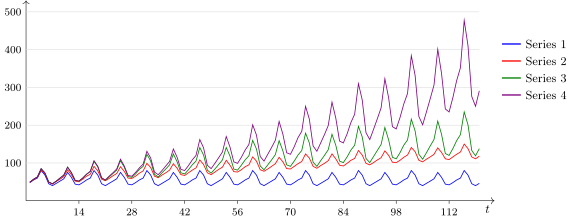
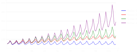
The same device on a conventional two-week profile of period 14: series 1, ; series 2, ; series 3, ; series 4, .
To get some intuition, let us look with our own eyes at what trends and seasonalities are. I have drawn here a bunch of model time series: I took a pattern of 14 points, two weeks long, and began repeating it. If it simply repeats as a periodic function, that is series 1: there is seasonality, we know the period, we set 14, and there is no trend, the average level does not shift anywhere over time. Series 2 is when there is a linear trend: we do not simply repeat the seasonal profile as a periodic function but also add a linear function; it is the sum of a linear function and a periodic one.
Series 3 is a linear trend, but the seasonality is multiplicative: we do not add but multiply. Multiplicative seasonality occurs very often precisely in econometric processes, because many processes in economics, as in biology or ecology, are arranged so that the rate of change of some quantity is proportional to the quantity itself. Such a differential equation gives solutions similar to an exponential, and such proportionality itself is built into many effects. For example, if you increase production by 15 percent every year, that means an exponential: growth of 15 percent year after year is exactly an exponential. And within a year there may be a yearly profile: more is produced in summer than in winter, because of weather conditions, say. This is a typical case where you will have both an exponential trend and multiplicative seasonality (series 4), because the whole production process is arranged proportionally: so many times, so many percent less or more is produced.
Here are two kinds of trend — linear and nonlinear — and two kinds of seasonality combined with this trend — additive and multiplicative. These cases are the most common in practice; it is such series that we observe most often. And of course monotone trends never go on forever. Any processes first develop, grow, then enter some stagnation — something like stationarity appears — and then begin to fade: they lose the competition, for example, or something else happens to them. Trends are not eternal, and this too is an important point that one has to learn to use somehow. Any trend has some lifetime, a duration during which this model works, and then it starts to work worse and worse, or the trend parameter starts to change, or something else happens. One has to be able to adapt to these changes. The time series model itself may be simple, but it must be able to adapt to changes of this kind.
The Holt model
Definition (The Holt model). A linear trend without seasonal effects:
where , are the adaptive coefficients of the linear trend.
The recurrence formula:
where are the smoothing parameters.
Let us see how such models are arranged. There is a whole series of models here; they are all called adaptive short-term forecasting models. The simplest is the Holt model: a linear trend without seasonal effects. Let us compare with what we did in the exponential moving average: there we said our regression model is as simple as can be, a constant. How can this model be enriched with a trend? Very simply: let us say that it is not a constant but a linear function of time — more precisely, of how many days ahead we want to make the forecast; time enters here as the forecasting horizon . The main thing is that two parameters appear in the model, and . Why do they have the index ? We want them to be adaptive, so that the trend formula can change over time. This is exactly what I said: for some time our trend is increasing, then it may become decreasing, and this will show in the sign of . The main thing is that we can find and at each moment from the history of the series.
This model is a little more complex than the previous one, where there was simply a constant; the previous one is its special case, . So exactly the same trick can be done with it. I will not write out the calculations, but here is what we do: instead of we substitute , differentiate with respect to the two parameters and , set the derivatives to zero and get a system of two equations in two unknowns. We solve this system and, just as before, get a formula that expresses through the history of the series. Now we write this formula for the moments and and express one through the other recurrently. The scheme is exactly the same; the only difficulty is that before we solved one equation for , and now a system of two equations in two unknowns.
We get recurrence formulas that, if you look closely, differ in nothing special from the previous case: this too is an exponential moving average, but with its own smoothing parameters, and here there are already two of them. We can of course set them equal to each other, but we can say that the slope of the trend has one speed of adaptation and the free term another; in principle we have the right to do so. So for generality and may differ. These are smoothing parameters, and their meaning is the same as before: if the are small, the series looks stationary; if the approach one, the model starts to adapt faster. And it is easy to see that if , we automatically get the previous case.
The Theil–Wage model
Definition (The Theil–Wage model). A linear trend with additive seasonality of period :
is the trend cleared of seasonal fluctuations; is the seasonal profile of period , without trend.
The recurrence formula:
where are the smoothing parameters.
Now let us deal with seasonality. Let us keep the linear trend: it is neat, especially since it adapts, its own and are determined at each moment, and that is great. That is, we do not just have a linear trend over the whole history of the series: at each moment it is a little different from the previous ones, and in the end it turns out nonlinear. To this linear trend we want to add seasonality. Suppose we understand that our function is quasi-periodic, and we know the period — this is very important. In most cases it is the number of hours in a day or the number of days in a week, that is, we always know it. Situations where there is a periodicity with an unknown period we do not consider at all — that is a more complex case.
What must we do? The seasonal profile simply has to be repeated. How can this be done? Very easily — by adding , more precisely : simply by changing the index we refer to the array of values from the last period and never refer to an index from the future — this is exactly what this formula guarantees. We simply add one of these numbers to our linear trend, and which one exactly the index tells us. To be definite — the day of the week: the period is then 7, and if we make a forecast for Wednesday, we must take the previous Wednesday into account.
How many parameters are in this model? . We must again carefully write out the least squares functional, differentiate with respect to the parameters, with respect to , and all the , set the derivatives to zero, get a system of equations and solve it — it splits into independent equations, and the solution is very simple. In the end we get these three recurrence formulas. The formulas for and are very similar to the previous case, except that when we estimate the trend we subtract the seasonality — we clear the trend of seasonality, and when we compute the seasonal profile we clear the time series of the trend. This is already interpretation: clearly the formulas are derived from solving the least squares problem, but looking at them it is easy to understand what is going on here. In estimating the seasonal profile we try to clear the time series of the trend, and conversely, in estimating the trend we clear the series of the seasonal profile. These models really are often used in forecasting sales volumes and in various other problems.
The Winters models
Definition (The Winters model). Multiplicative seasonality of period :
is the seasonal profile of period .
The recurrence formula:
where are the smoothing parameters.
So far these were linear models, and here is an example of a model with multiplicative seasonality. Let it be without trend for now: there is simply some constant, as in the exponential moving average, but we want to throw a seasonal profile onto it, also of period . Then we simply change the plus here to a multiplication. How to work with such time series? In fact very simply: take their logarithm, then the multiplication turns into a plus, and pose the least squares problem for the logged series. But this is only a sketch of a proof; I do not want to go into the details today of how all this is derived — these are all not very hard exercises. And the recurrence formula works in a quite predictable way, only now clearing the time series of the seasonal profile looks like this: if before we subtracted the seasonal profile from , now we divide by the seasonal profile. That is the whole difference. And in the same way, to estimate the seasonal profile, has to be divided by rather than subtracted. Such a model is used when there is an initial assumption that the time series has a multiplicative effect.
Definition (The Winters model with a linear trend). Multiplicative seasonality of period with a linear trend:
is the trend cleared of seasonal fluctuations; is the seasonal profile of period .
The recurrence formula:
where are the smoothing parameters.
A linear trend is easily added here too — the Winters model with a linear trend. Click through the slides and spot the differences: we took the constant that was here before and replaced it with a linear trend; that is the main difference. Then we do all the same things: where we need to get rid of multiplication, we take logarithms, and the recurrence formulas are derived without difficulty. Clearly in some places there will be division and in others subtraction: the trend is linear, so in the formula for the slope there is subtraction, while the seasonal effect is multiplicative, so clearing it is division. This is a rather obvious interpretation, but, I repeat, the formulas are derived rigorously.
Definition (The Winters model with an exponential trend). Multiplicative seasonality with an exponential trend:
is the exponential trend cleared of seasonality; is the seasonal profile of period .
The recurrence formula:
where are the smoothing parameters.
And finally one more model — the Winters model with an exponential trend. Now, instead of making a linear trend , we multiply by to the power . Again, by taking logarithms everything reduces to the additive case, the least squares method is written out, and the recurrence formulas are derived.
In fact a number of further such models can be churned out. Nested seasonal profiles can be taken into account if necessary — when days nest within a week, or something else of this kind happens. Some more complex trend models can be taken into account. But in the problems I have told you about, you will hardly ever have to build trends more complex than linear ones. Even if , adaptation still produces rather non-trivial modelling.
The adaptive autoregression model
Definition (The adaptive autoregression model). The linear autoregression model (a linear filter):
is the error of the forecast made at step .
The least squares method: .
One step of gradient descent at each moment :
The gradient step in the steepest descent method:
where is an analogue of the smoothing parameter.
What else non-trivial can be arranged, apart from these simple adaptive methods, which are slightly generalised exponential moving averages? Let us go back to the linear autoregression model, or the so-called linear filter. Can a recurrence formula be made from it too, so that the coefficients adapt? It can, but we come at it from a completely different side, and the result turns out very similar to the previous models.
Let us simply apply the gradient descent method: the next observation has come to us, and we take a gradient step to minimise, say, the squared error. So step by step, for each moment , one step of gradient descent. It is very easy to write out: it is a small change of the parameter vector, where is the -th parameter, and the features, as we agreed for autoregression, are the previous values of the same time series. Hence, by the way, the name "autoregression": we build a regression model from data contained in the history of the time series itself.
Moreover, the least squares problem is wonderful in that it is solved analytically, and the optimal step can even be determined by the steepest descent method. There is this formula for the optimal step, where can in principle be set to one, but it can also be chosen — so as to turn it into an analogue of the smoothing parameter. Clearly, the smaller , the less we adapt our model, the more confident we are that our original series is stationary — the very same story as with the smoothing parameters.
Remark (A question: once more about the adaptive linear filter?). Let us go back once more to the autoregression problem. What happens when the next element appears in the time series? We have to add a row to the matrix and one more element at the bottom of the vector , and in principle solve the problem anew. But we do not want to solve the problem anew, because that takes a lot of time, especially since the matrix has changed by only one row. Probably one can recompute the solution relying on the already known one; such a method may exist too, but I have not written it out here in detail — it is computationally more expensive.
Or, when one more element of the time series is added, one can simply take one step of gradient descent to modify the parameter vector taking into account the new point that has just arrived. That is what we do. We introduce the forecast error for the new element of the series: yesterday, at step , we made a forecast for today, and when today's value has appeared, we can already compute the error. We minimise the squared error over the parameters . This is very similar to the stochastic gradient method: we minimise not over all at once but only for one . But unlike the stochastic gradient method, where we choose objects at random, here time flows sequentially, and each time we take the next sample of the time series: day has come, we have learned the forecast error and now can minimise over . The parameters sit in , and here is what one step of gradient descent looks like: we honestly differentiated with respect to , and the derivative is multiplied by the corresponding feature, that is, by the value of the series that stands at in the forecast . Differentiating is very easy.
Then we take this gradient step, and it turns out to be very similar to our adaptive steps. Moreover, an analogous smoothing parameter with an analogous meaning can be used here: the smaller , the less we adapt the vector , the more stationary our series. And clearly this too would have to be optimised here by cross-validation, as we have already said.
Analysing the adequacy of adaptive models
The tracking signal
Definition (The tracking signal). is the error of the forecast made at step .
The tracking signal [Trigg, 1964]:
is the EMA of the error; is the EMA of the absolute error.
Recommendation: .
A statistical test of adequacy (for , ): the hypothesis : , is accepted at significance level if
is a quantile of the normal distribution; for .
Let us go on: we will gradually complicate things and look at more and more interesting approaches to forecasting. Here is one more thing, very useful for checking how adequate our time series model is — the tracking signal. It is often used precisely for choosing models: to understand which models are adequate for forecasting a given series and which are not.
Let us look once more at the error — exactly the quantity we introduced on the previous slide: the forecast was made yesterday, today has come, we have seen the true value and can now understand how much we erred yesterday. The tracking signal is the ratio of two exponential moving averages: the first is the EMA of the error itself, the second the EMA of the absolute error.
If the time series is modelled well and the model has no systematic biases relative to the truth, the signs of the errors keep jumping across zero: the error is now less than zero, now greater. When we average the themselves, we have many small positive quantities and many small negative ones, and as a result their mean tends very nicely to zero: the large and small ones compensate each other. That is, if the model is good, the EMA of the error should tend to zero. But the EMA of the absolute error does not tend to zero: if we start smoothing the absolute values by an exponential moving average, it tends simply to the mean deviation of the errors. If the tracking signal tends to zero, that is very good: the errors are now positive, now negative, and most likely the model is unbiased or close to unbiased, that is, it is a decent model. The smaller , the better; and cannot be greater than one: since the numerator has the errors and the denominator their absolute values, is bounded by .
We are going to use this quantity to understand how adequate our model is: we watch how well the errors behave. This is a kind of residual analysis — errors are also called the residuals of a regression model. But since an exponential moving average is used here, the question arises: what should its smoothing parameter equal? There is a more or less standard recommendation, from five hundredths to one tenth. This means that we average over roughly the last 10–20 measurements, and one need not worry much about choosing . We will see in a moment how the tracking signal is used to choose the smoothing parameters, those very , but in this quantity itself can be fixed.
How is used in a statistical test of model adequacy? What is an adequate model? It is a hypothesis , which in this case consists of two theses: the model is unbiased, that is, the expectation of the errors is zero, and there are no residual correlations between the at different moments, that is, we have taken into account all the dependencies that were in our data. This hypothesis can be tested with such a statistical test; are quantiles of the normal distribution. We approximately describe the distribution of the random variable — the statistic — by a normal distribution, and the variance of this distribution turns out to be related to . We get such a formula through quantiles of the normal distribution. If the significance level is fixed, five percent, then can be taken as roughly two; it is not a very large quantity. And we accept the hypothesis at the given significance level if is small enough.
Remark (A question: what is a significance level?). You have not had mathematical statistics yet? So that is the thing. I will not give you a lecture on testing statistical hypotheses now, but in two words: what is testing a hypothesis? You set some probabilistic assumption — in this case there were two: that the expectation of the errors is zero and that they do not correlate with each other. Under these probabilistic assumptions you derive the distribution function or the probability density of some statistic; in our case the statistic is the random variable . A statistic is, formally, a measurable function of the sample, that is, something we can compute from the sample. In general the methodology of testing statistical hypotheses is very broad: a very wide range of probabilistic assumptions, which we call the hypothesis and test, and a very wide range of statistics — numerical quantities that can be computed from a finite sample. A statistic is any numerical quantity that can be computed from the sample: if you like, the mean; if you like, the exponential moving average. The main thing is that for this random variable you must derive the probability density analytically under such-and-such probabilistic assumptions. Here one has to apply probability theory; this problem is sometimes very hard, sometimes not very, but it is solved analytically, and as a rule the form of the distribution is derived asymptotically. In this case the asymptotics is a Gaussian distribution.
And then the following happens. You have derived the probability density of your statistic and say: if all is well, the hypothesis holds, then what values of the statistic are expected? Values close to zero — good. But what if the value of the statistic suddenly became very large? What "very large" means is that it fell into the tail of the distribution, in this case the right tail, where the values are large but improbable. If an improbable value of the statistic has occurred in practice, this means that the observed sample does not match the hypothesis , and we say: the data do not confirm the hypothesis . If, on the other hand, the value of the statistic fits well into this distribution, has not flown off into the tails, its value is quite probable, then we do not reject the hypothesis: the data do not allow us to reject it. In our case we say that the model is adequate: if the observed value of the tracking signal is small enough, it is quite consistent with the hypothesis. In testing statistical hypotheses nothing can ever be asserted for certain.
So, the significance level is that small probability concentrated in the right tail of the distribution. We can put a cut-off and say that to the right of it the probability is five percent; then these five percent are the significance level. If we have landed in that very five-percent right tail of the distribution, we will reject the hypothesis , that is, assert that our data are not consistent with this hypothesis.
Remark (A question: why does the statistic use a moving average rather than the errors over the whole interval?). This is an arbitrary choice in constructing the statistic. Generally speaking, we could have done as you suggest; moreover, if the series is stationary, that is exactly what should be done. But if the series is non-stationary, its deep, distant history may no longer have anything to do with the current behaviour of the series. We count on being able to work with both stationary and non-stationary time series with a single approach, and for this exponential moving averages are convenient: if the series is stationary, can be made very small; if non-stationary, larger, but in principle not too large. One tenth is the most frequent recommendation.
The Trigg–Leach model
Definition (The Trigg–Leach model (Trigg, Leach, 1967)). The problem: adaptive models adapt poorly to sharp structural changes.
The solution: .
Drawbacks:
- it reacts poorly to single outliers;
- has to be chosen, with the recommendation .
What is the tracking signal used for? There is such a model — the Trigg–Leach model. It is rather old, but when we were solving problems of forecasting consumer demand, many of our customers had on their desks Lukashin's book "Adaptive Methods of Short-Term Forecasting" — it is already almost twenty years old, and I refer to it here several times too. And all these old methods, developed in the 60s–70s, nobody has cancelled: they are actively used, they are quite adequate, simple, and quite sufficient for solving many practical problems. One of these methods is designed for handling sharp changes of model — for detecting that a time series has somehow abruptly become non-stationary.
An artificial series with a jump in the mean level: Brown's model (exponential smoothing) takes a long time to catch up with the new level, the Trigg–Leach model adapts to it quickly (slide).
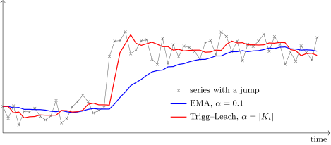
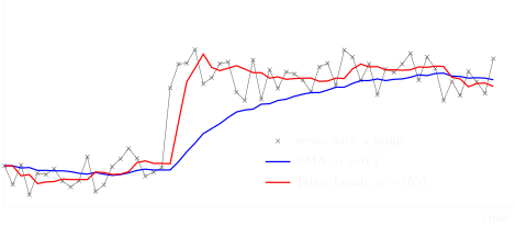
A model series with a jump in the mean level at the moment : the EMA with constant takes many steps to catch up with the new level, the Trigg–Leach model with () reaches it in a few steps.
An example is shown here. There is the original time series, shown by crosses, and we build some exponential moving average model, of the Brown model type. What do we see? The series first had one mean level, then jumped sharply to another mean level — this is an example of a change point: a change of the time series model has happened here. What will a simple exponential moving average model with a fixed smoothing parameter do? It will take a long, long time to catch up. And what one would like to do at this moment is to increase the value of the smoothing parameter : the series has become non-stationary; at this moment and the following ones we can no longer say that it is stationary, so must be increased.
Which quantity lets us say that the series has abruptly become non-stationary, that is, will increase at such a moment? It is the tracking signal. Look at what happens here. The ordinary exponential moving average model starts to take a long time catching up with the original series, and a systematic bias arises: all the errors are positive, , the original series lies higher than our forecasts . And what will happen in the exponential moving average of the errors? We will start averaging values that are positive all the time; they will start adding up instead of positive and negative ones compensating each other all the time, as it was before. And will grow quickly. The idea of the heuristic is simply to take this current as the smoothing parameter , because behaves exactly as we would like to: as soon as the series becomes non-stationary, we want to increase , and behaves exactly so. The Trigg–Leach model is nothing more than this heuristic: let us take the smoothing coefficient numerically equal to the tracking signal. That is what makes it useful.
Adaptive selection and composition of models
The idea of adaptive selection
The dynamics of the EMA of the forecast errors for 6 models (on real data of sales volumes in a supermarket). The idea: it seems one can manage to switch on the most successful models and switch off the less successful ones in time.
Let us move on to one more very good idea — we are gradually complicating our methods. This is the idea of selection, or composition, of models. Here I show what the time series of errors look like — more precisely, of the absolute errors — for six models. We took one and the same time series and six different models. We have probably already gone through more than six models, starting with Holt and Winters, the adaptive linear model, and in general there are in fact dozens, hundreds of them. One can try to forecast one and the same series with different models and try to detect intervals of time where one model or another works well, and thereby detect the moments when the model changes — find a change point.
Here is just an example that shows that there are intervals where the thick black model works worse than the others, there is a rather long interval when it works better than the others, and there is a rather long interval when all six models are practically indistinguishable from each other — they work the same, by the way, equally badly. Can we manage to switch on the most successful models in time, as soon as we detect that a model already systematically gives smaller errors than the others? This idea is very easy to implement.
The adaptive selective model
Definition (The adaptive selective model). Suppose there are forecasting models; is the forecast of the -th model for the moment ; is the forecast error of the -th model at the moment ; is the EMA of the absolute error.
The best model at the moment :
The adaptive selective model is the forecast by the best model:
has to be chosen; the recommendation is .
Suppose we have forecasting models, and we build the forecasts of the -th model for the moment — everything as before, only now there are several models, runs from one to . For each model we define the forecast error and take the exponential moving average of the absolute error. The tracking signal could be used here too, but one can make do with simply the exponential moving average of the absolute error. What is the best model? The one whose is the smallest at the current moment: is the number of the best model at the moment , because its mean error is the smallest.
Then it is clear what to do: since we have determined the best model at the moment , let us use the best model for the forecast for the moment . The adaptive selective model is simply the forecast by the best model. The formula came out a little convoluted, with three-storey indices, but very simple and understandable: is the index of the best model, and the forecast of our whole composition is built by the best model at the moment . That is all, a completely simple selection model. It too is adaptive, and it has one parameter — this very — which can also be chosen. These smoothing parameters keep arising, but we know what to do with them: they have to be chosen by cross-validation.
Adaptive composition of models
Definition (Adaptive composition of models). Suppose there are forecasting models; , , are as above.
A linear (convex) combination of the models:
Adaptive choice of the weights [Lukashin, 2003]:
has to be chosen; the recommendation is .
But selection is not the best idea, and one can move from selection to composition. Look, we start with the same thing: we have models, we build the forecast errors for each model and the exponential moving average of the absolute error. But now we do a slightly different thing. Instead of choosing one best model, we say this: what if among the models there are several best ones, several decent ones? If we select these decent models and average their results, then probably our forecasts will be more reliable, because they are as it were made by a vote of several models.
This idea too is very easy to implement. We set the forecasting model as a weighted sum, a linear — more precisely, even a convex combination of the forecasts given by our individual models. We took some weight coefficients, non-negative, summing to one, and added up our models with these coefficients — in effect we made a composition, a linear adaptive composition of models. The question arises of how to choose the weights . There are a pile of different formulas here; one of them is in Lukashin's book. Clearly, the smaller the error, the larger the weight, that is, the more reliably the corresponding forecasting model works. So we can take any continuous decreasing function and apply it to the errors; here a hyperbola is taken, but something else could have been taken. Then it has to be normalised, since the sum of the weights must equal one.
Remark (A question: what happens if the error suddenly becomes zero?). From the practical point of view, first, this is of course rare. Second, one can always add to the denominator and solve this problem with zero. But I assure you, it happens extremely rarely: the denominator has a sum over all the models, and if a zero came out there, this means that all the models are ideal and made no error at all. In practice such a situation is hardly realisable.
Although you are of course right: there are degenerate situations. For example, a zero time series can very easily come out if we forecast hundreds of thousands or millions of time series — and the range of goods in a supermarket is on the order of a hundred thousand, and nobody of course checks that all the data are clean and non-degenerate. Suddenly there is a product that has been entered into the database but has never been sold; then the time series is pure zero, all reasonable models will look at this series and say "zero" in unison — they are not fools. And your situation really does occur. There is a very simple trick against zero: let us add some small to the denominator. If we want the coefficients to be normalised, it has to be added to both the numerator and the denominator.
LAVR, local adaptation of weights with regularisation
Definition (LAVR, local adaptation of weights with regularisation). At each step the weights are determined by least squares and smoothed:
is the coefficient of "forgetting" the history; is the regularisation coefficient.
Additional variants:
- : local adaptation of weights with regularisation (only one term is left in the functional, );
- : a monotone corrector.
K. V. Vorontsov, E. V. Egorova. Dynamically adaptable compositions of forecasting algorithms. Iskusstvennyi intellekt, 2006 (in Russian).
And finally I will tell you about one method that we devised fifteen years ago, just when we were working on problems of forecasting sales volumes. We called it LAVR, local adaptation of weights with regularisation; it is the acronym of the method's Russian name. We liked it enormously, because it turned out to be simple and at the same time beat all sorts of other methods very impressively. So let me tell you about it.
The idea is this: still use the least squares method. It is a linear model, as before — a convex combination of models, an adaptive composition: we have the original models, the -th model at the -th point gives the forecast , and there are weight coefficients we want to adapt. Written out here is exactly the least squares criterion that we usually use when deriving the exponential moving average: there are weights of the objects — the objects here are moments of time — which decrease exponentially into the past. If this problem is solved head-on, then at each moment one has to solve a problem whose solution time is cubic in the size of the data; that is of course unpleasant.
And an important point is the regulariser. Regularisation says that we do not want the coefficients to change by jumps, very abruptly: if they change abruptly, this lowers the stability of the model. The main assumption here is that some switching of the model is unlikely to happen every day. If a model works, it worked yesterday and will work tomorrow, perhaps a little worse, but at least the coefficients should not jump very strongly every day. So we stabilise them with such a regularisation. In time series forecasting in general this is a rather frequently used construction of regularisation. Here is the coefficient of forgetting the history, the regularisation coefficient.
What additional variants do we have in this model? The first: if we let tend to zero, we will be doing precisely local adaptation of the weights. Letting tend to zero, we in effect keep only one term out of from to — all the others, except the last, will be absent. On the one hand, this is very similar to the adaptive autoregression model, when we shift the vector on the basis of only the one last observation. But there a gradient step was used for this, and here we will do it differently. The model is also linear, very similar, but we will solve the least squares problem with only one term and force the solution obtained to be close to the solution we got at the previous step. In this way, instead of training on the whole training sample, we will train only on the last moment of time — on one point instead of points — but at the same time force the solution to be close to the previous one, and a certain continuity of solutions will still be maintained. We did experiments in which we looked at whether can be let tend to zero or whether the heavy problem on the full training sample has to be solved. And one more possibility we tested is whether it makes sense to impose non-negativity constraints on the coefficients , or whether everything will work well without them.
Experiments with adaptive compositions
The problem of forecasting sales time series: the mean forecast error on cross-validation () as a function of the logarithm of the regularisation parameter. LAVR-M gives the best result, and can be taken; the monotonicity constraint is a strong regulariser.
Let us see what comes of this. Here is one of the examples of how the methods performed. Our best method turned out to be local adaptation of weights with regularisation and a monotonicity constraint. Plotted here is the mean forecast error as a function of . Why is this constraint called monotonicity? Because a convex combination with non-negative weights is monotone in its arguments: the larger these , the larger the response of our linear composition.
And it turns out that the monotonicity constraint is in itself such a strong regulariser that can be let tend to zero: we no longer need to stabilise the coefficients relative to the previous ones. This is a very amusing effect: the horizontal part says that can be taken very small, let tend to zero (the logarithm of is plotted on the horizontal axis), and that turns out to be the best solution of all. That is, one can let tend to zero and take equal to zero if we impose the monotonicity constraint.
Fragments of the dynamics of the weights of the base models: without the monotonicity constraint (top) and with the monotonicity constraint (bottom).
And one more illustration. If we switch on the monotonicity constraints — here there are a number of models, and here are the weights they take — then at each moment we in fact use a small number of models, as a rule one, two, three, but no more. Without the monotonicity constraint, one can see that some of the models play as it were against themselves all the time. We tuned the individual models, these are also adaptive forecasting models, they must forecast the original series, and yet in the linear composition we for some reason take them with negative weights. This somehow does not correspond to common sense. But if we start imposing non-negativity constraints on the weights, we see that many models simply switch off; their weights are zero. This is a very amusing effect.
Remark (Comparison of models). The mean forecast error on cross-validation ():
| Base models | Error | Compositions | Error |
|---|---|---|---|
| base-1 | 0.7142 | LAVR + Monot | 0.5899 |
| base-2 | 0.7294 | selection + smoothing, | 0.5956 |
| base-3 | 0.7534 | LS + Monot, | 0.6314 |
| base-4 | 0.7624 | LAVR without Monot | 0.6591 |
| base-5 | 0.7624 | LS without Monot, | 0.6834 |
| base-6 | 0.7664 | LS on all data | 0.7142 |
| base-7 | 0.7793 | mean | 0.7294 |
| base-8 | 0.7793 | selection without smoothing | 0.9107 |
- The base models, their averaging, non-adaptive least squares on all data work poorly.
- Adaptive selection works well if is chosen: , averaging over 3…5 days.
The main thing is that the method of local adaptation of weights with regularisation and with the monotonicity constraint very often gives the best result of all. Here we used eight base adaptive forecasting models, made linear combinations of them, and compared which strategy of linear combination works best. We understood that regularisation rules, and that monotonicity is in itself a very good regularising constraint. The second model in this list — selection plus smoothing plus the optimal choice of — also works quite well in this particular problem. But complications of the problem — when we take non-zero or also optimise — work worse. And what we achieved here: the combination of models performs even better than the best base forecasting model. The best base model has an error of 0.71, and we reduce it almost to 0.6.
Summary
Remark (Summary).
- Adaptive methods are used when there are many series and they have to be forecast quickly.
- Simple adaptive methods are strengthened by adaptive selection and composition of models.
- Simple features of the series (trends, seasonalities, gaps) are modelled in the base algorithms.
- The monotonicity requirement for an adaptive composition is a powerful regulariser.
- More complex dependencies are modelled by adaptive autoregression models.
Yu. P. Lukashin. Adaptive Methods of Short-Term Time Series Forecasting. Finansy i statistika, 2003 (in Russian).
We have come to the end. There are of course cool forecasting methods — ARIMA, neural networks and so on. But the question is: why use a sledgehammer to crack a nut? Especially if you need to forecast a hundred thousand time series and do it on a modest server of some large retail chain within a two-to-three-hour window at night — rebuild all the forecasts for the next day or the next week or two. These forecasts are needed for making purchases. And clearly retail is not the kind of client that will put up a supercomputer centre to compute some forecasts. That is, the methods must work very fast, and so adaptive methods like the ones I told you about today are very good.
They must take into account rather simple effects: trends, seasonalities, zero intervals, promotions and holidays — that is practically everything that has to be taken into account in this problem, and it is very easy to do with different models. And then one has to take into account that goods abruptly change their behaviour from time to time: either a competing product has appeared, or the supplier has changed, or something else has happened. We will of course never detect such effects by hand on a hundred thousand time series. The model has to be adaptive, or rather, there should be several models that can switch between each other adaptively. And in such applications the "adaptive selection and composition" approach turned out to be the most successful. That very book by Lukashin that I have advertised — the reference is below; it is rather old, but it still remains the forecasters' desk book.
Remark (A question: why do negative weights appear in LAVR without the non-negativity constraint?). We either use the non-negativity constraint or we do not: we simply investigate both variants, because a priori we do not know which is right. When we tried both variants, it turned out that the non-negativity constraint really is necessary. If it is not used, the problem itself has such a solution, and this solution is not very sensible: here we have six models, some of which have negative coefficients and some positive. It looks altogether like some kind of overfitting. We tune each of these models separately so that it forecasts one and the same time series, and suddenly, when we start adding these models up, some of them pop up with a negative coefficient. What does this mean? The model in the composition as it were works against itself: it takes its forecast with a minus sign. This cannot be interpreted in any way.
No comments yet
Be the first to share your thoughts.