August 30, 2026 · Lecture · LibreTimes
Machine Learning 2. Lecture 1. Deep Neural Networks
Contents
- What this lecture is about
- Reminder: neural networks and their training
- Vanishing and exploding gradients
- Dropout and batch normalisation
- Deep neural networks and their justifications
- Depth matters more than width
- Feature generation and end-to-end learning
- Convolutional neural networks
- The convolution layer
- The pooling layer
- The standard scheme of a convolutional network
- AlexNet: a convolutional network learns to extract features
- ImageNet and the deep learning revolution
- ResNet: the residual neural network
- Convolutional networks for speech, texts and games
- Recurrent neural networks
- Sequence processing problems
- Training recurrent networks: BPTT
- Long short-term memory networks (LSTM)
- Variants of LSTM and GRU networks
- Conclusions
- Seminar
What this lecture is about
Good afternoon, and welcome to the second half of the course on machine learning. We present it as two semesters: last semester was the mathematical foundations, and this one is applied models. The difference is this: we will talk a great deal about neural networks and about various applied problems, where the applied side will come to the fore and constantly affect how we build our models. I want to begin this part with neural networks: for the first few lectures we will be dealing with neural networks.
Today, two types of deep neural networks that are in a sense considered the main ones, although a huge number of neural network architectures have been invented by now: convolutional neural networks, which came from image processing, and recurrent neural networks, which come from the processing of signals and texts. But first a short run, literally ten minutes, through last semester's lecture on neural networks: we will constantly refer back to the things that were told there.
Reminder: neural networks and their training
Definition (The mathematical model of a neuron (1943)).
where are the features of the object ; are the feature weights; is the activation threshold; is the activation function.
The model of a nerve cell, a neuron, works like this. If is a feature vector (in the input layer of a neural network) or the vector of outputs of the previous layer (in the intermediate layers), then in each neuron we compute a linear combination of these features with synaptic weights , the trainable parameters. Since there are many neurons in a layer, the weights form a whole matrix.
Definition (A multilayer network: MLP (MultiLayer Perceptron) with layers). The network architecture: is the number of neurons in the -th layer, ;
- is the feature vector at the input of the network, ;
- is the vector of "features" at the output of the -th layer, ;
- is the vector at the output of the network;
- is the weight matrix of the -th layer, of size ;
- is the layer-by-layer computation of the network, .
The size of a layer's weight matrix is the number of neurons by the dimension of the input vector. A fully connected two-layer network is the picture we looked at when we began working with the backpropagation algorithm. Backpropagation is our everything: with the error backpropagation algorithm we train not only simple fully connected networks but also deep neural architectures — regardless of how many layers there are, how many neurons are in each layer, whether all the connections are present or we introduce only some of them by means of constraints. We will now see how this happens with the example of neural networks for image processing. Imagine that the picture with two layers continues, and take as many layers as you need.
Definition (The SG algorithm (Stochastic Gradient)). is the loss incurred by the model on the object . The criterion of the minimum mean loss on the training sample:
Input: a sample ; learning rate ; parameter . Output: the weight vector of all layers .
- initialise the weights and the current estimate ;
- repeat
- choose an object from (for example, at random);
- compute the loss ;
- gradient step: ;
- estimate the value of the functional: ;
- until the value of and/or the weights stabilise.
H. Robbins, S. Monro. A stochastic approximation method. Annals of Math. Stat., 1951.
The stochastic gradient algorithm is our second everything; or rather the first, and backpropagation is a special case of this algorithm, a particular way of computing gradients. The main thing: we choose objects one at a time at random, take a gradient step on each object, pass through all the objects many times — that is what training consists of. In more advanced algorithms this logic gets more complicated: nobody has taken objects one at a time and stepped along the gradient of each for a long time now; there are many tricks for speeding up the gradient method.
Definition (The method of accumulating inertia (momentum)). Momentum is an exponential moving average of the gradient over the last iterations (B. T. Polyak, 1964):
NAG (Nesterov's accelerated gradient) is an accelerated stochastic gradient with inertia (Yu. E. Nesterov, 1983):
There is the method of accumulating momentum, which in Russian is often called the "moment" — but it is not a moment at all, it is momentum. In effect what is computed here is an exponential moving average of the gradients: the gradients from previous iterations are taken with weights that decrease into the past. The gradients from previous iterations can be aggregated in different ways. One can form so-called batches, subsets of objects (they are sometimes called mini-batches; sometimes a batch is split into mini-batches), and average some things over some and other things over others. All this is aimed at averaging the gradients so that they show us the direction in which the functional decreases more clearly, so that we move faster and each individual object does not pull us aside from the general direction of motion.
Vanishing and exploding gradients
Another problem is exploding or vanishing gradients; they are usually mentioned together. If we put many layers one after another, then when computing the gradient in a multilayer network we compute derivatives at each layer, and then in effect they are multiplied together. If numbers less than one are multiplied all the time, the derivative ends up tending to zero, and we cannot move from the dead point we have landed in; this is also called the problem of network paralysis. If, on the contrary, the derivatives are greater than one, they multiply and accumulate — that is the problem of exploding gradients.
There are several remedies for exploding gradients. A very simple one is gradient clipping, where we simply forbid the gradient to be larger than some constant . Not the best way; there are more interesting ones.
Definition (Activation functions). The functions and can lead to vanishing gradients or "network paralysis".
The positive part function (Rectified Linear Unit, ReLU):
One of the most frequently used ways is to give up sigmoid functions and all other functions with horizontal asymptotes. It turns out that if we replace them by a piecewise linear function equal to in the positive region and zero in the negative one — its derivative is either exactly zero or exactly one — then neither vanishing nor exploding gradients can happen in principle. The gradient can become zero, and that is even good: if we see that we have landed in the negative region, we can even save on computation — why compute this zero and add it.
Dropout and batch normalisation
Another interesting trick that turned out to be very useful precisely in deep neural networks is dropout. It is a kind of regularisation. Dropout is done on mini-batches: we take a certain number of objects together and say that we will train the neural network on them, but we randomly refuse to use a certain subset of the neurons. On each mini-batch a new random subset of neurons is generated, which we train, and the rest are discarded. What does this mean? That we train the network to be super-robust, that is, in a sense we copy a feature of natural neural networks, their very high reliability. If some number of nerve cells switch off for some reason — they are damaged, have stopped functioning, are in a state of long relaxation — nothing terrible happens to brain activity: the other neurons take over their role, the functions are heavily duplicated. For this to happen, the neural network has to be trained accordingly, and a simple way to achieve a lot of duplication in a network, and hence high reliability, is dropout.
Another useful trick is batch normalisation. It would seem a very simple trick, but it makes it possible to get rid of the accumulation of all kinds of computational errors. For more than half a century, since the fifties and sixties, machine learning has favoured the trick of normalising the vectors fed to the input of a neural network or some other algorithm: for example, normalising an object's feature description by the Euclidean norm so that it equals one. This usually makes a method more computationally stable. The idea of batch normalisation is to normalise not only what comes into the network's input but also the outputs of each layer: the vectors going from one layer to another are normalised again. Normalisation requires computing certain coefficients, and it happens by batches: we split the whole large sample into batches, and each batch gets its own normalisation. After the normalisation one has to put a simple linear transformation with tunable weights — in essence one more small linear layer. Practically all modern deep neural architectures are tuned using batch normalisation.
We have deliberately gone through only the tricks that turned out to be very important when the number of layers began to grow: they improve convergence and make it possible to keep adding layers.
Deep neural networks and their justifications
Definition (Deep neural networks (Deep Neural Network, DNN)).
- 1965: the first deep neural networks.
- 2012: the convolutional network for image classification AlexNet.
- The network architecture is the structure of the layers and of the connections between them, which makes it possible to give a DNN the required properties.
- DNNs make it possible to take complexly structured data as input and to generate it as output.
A. G. Ivakhnenko, V. G. Lapa. Cybernetic Predicting Devices. 1965 (in Russian). Krizhevsky A. et al. ImageNet classification with deep convolutional neural networks. 2012.
Depth matters more than width
A theoretical question was posed long ago: what matters more for the quality of training neural networks — increasing the number of neurons in a layer or the number of layers — in order to increase the descriptive power of this algorithmic family? What makes the number of functions we could in principle approximate grow faster: the number of layers or the number of neurons in each layer? A theoretical answer was given to this question: in 2016 a paper appeared that justified that increasing the number of layers leads to an exponential growth in the number of functions a neural network can describe, while growth in the number of neurons in each layer leads only to a polynomial one. So depth really matters.
Theorem (Depth matters more than width (Raghu et al., 2016)). is the family of fully connected multilayer networks : features, layers, neurons in each layer, , piecewise linear activation functions (ReLU, hard-tanh, etc.).
The measure of the diversity of the family is the maximum number of regions of linearity of , convex polyhedra in .
The diversity of the family grows as .
M. Raghu et al. On the Expressive Power of Deep Neural Networks. 2016.
Feature generation and end-to-end learning
Let us start with history. In image classification, before the neural network revolution, the accepted approach was this: first the images are preprocessed. If, for example, we are doing face recognition, the preprocessing consists of computing some features from the face: we pick out the oval of the face, the eyes, the distance between the eyes, the size of the nose, relative sizes on the face. A huge number of such features are invented, dozens. Clearly this is a specific thing: if you have learned to recognise faces well, it will not help you at all to recognise, for example, printed and handwritten characters, Chinese ideograms and so on. For ideograms you will have to build a feature system anew — and again put a whole department of engineers to work inventing geometric characteristics of the shape of objects in images. Each specific problem has its own feature system.
And there was a question: can an approach be invented in which the stage of feature extraction or feature generation is done fully automatically, and the feature extraction algorithms can be trained together with the recognition algorithm? This question received a definitive positive answer.
Remark (Feature generation for image recognition).
- The classical approach: hand-constructed image features, on top of which any trainable classifier.
- The modern approach, end-to-end deep learning: trainable neural image features and a trainable neural classifier; joint training.
Sanjeev Arora. Toward theoretical understanding of deep learning. ICML-2018 Tutorial.
An image is a complexly structured object that has no classical vector feature descriptions. Its structure is much more complex, and not only because it is a very large matrix of pixels. It would seem that each pixel can be described by three RGB numbers, and there is your feature description. But if we simply unroll the image into a vector, we lose a mass of information about the topology — about the fact that each pixel has neighbours. One has to learn to take this information into account somehow, and it seems critically important for image processing.
Convolutional neural networks
The convolution layer
How is preprocessing done for images in a way that turns out to be very universal for any images — regardless of whether you are recognising faces, cars or something else? These are convolutional neural networks. Convolution is an operation that has long and often been used in data analysis and machine learning. Convolution is in fact smoothing: if you have some data point and you know which points are its neighbours, you can average over them and get a smoothed value at the given point.
Definition (A convolution layer of neurons). are the original features, the pixels of an image; is the convolution kernel, , .
A non-fully-connected convolutional neuron with weights:
A little more formally: are the original pixels of the image, and we introduce a linear transformation that says: to get the value in the new, smoothed image, run over the whole neighbourhood of the pixel — of length and width and — and compute a linear combination with the weight matrix . The number of weights equals the size of the neighbourhood, the number of pixels in it, and each weight coefficient shows with what weight a particular pixel of the neighbourhood should be taken. Such smoothing produces a new, transformed image. This has been known for ages and is very often used for noise reduction in images. Recall nonparametric regression, the Nadaraya–Watson formula, kernel smoothing: exactly the same idea, only there the smoothing is over a one-dimensional structure, over a time series — we took neighbouring values and combined them with weights. Here it is the same, only the structure is two-dimensional, and you explicitly use the information about which pixels are close to each other: you have not lost this information, you know the neighbour on the left and on the right, above and below. The neighbourhood may be from to , or from to : it all depends on how large the images you process are and how large a neighbourhood you need to smooth over.
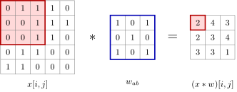
Convolution of a image with a kernel (; schematic, our example): the value in the highlighted cell of the result is the sum of the products of the kernel weights and the pixels of the highlighted neighbourhood, . Pixels at the edge, whose neighbourhood does not fit into the image, are not computed here, so the result is smaller than the original.
Fortunately, this structure corresponds exactly to a neuron: it is simply a linear neuron, in this form even without an activation function.
The pooling layer
Another interesting variant is the so-called pooling. In Russian I translate it as "combining neuron", although people go to various lengths to translate pooling, and, as far as I can tell, everyone just says "pooling".
Definition (A pooling layer of neurons). A pooling neuron is an untrainable convolution with stride that aggregates the data of an rectangular region:
where is an aggregation function: max, average, etc.
- The size of the image is reduced times in width and in height.
- If a neuron of the previous layer was responsible for detecting some element, max-pooling makes it possible to detect this element anywhere within an -neighbourhood (invariance of detection under shifts).
This too is a neuron, but its weight coefficients are not trained: it simply aggregates the values it sees in the given neighbourhood. Roughly speaking, you split the image into cells — for example , but the size can be whatever you set, even — and apply an aggregation function to all the elements of a cell. The first thing that comes to mind is averaging, but in practice the maximum works very well, max-pooling.
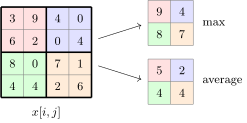
A pooling layer with (schematic, our example): each cell of the original image is replaced by one number, the maximum (max-pooling) or the mean (average pooling); the size of the image is halved in width and in height.
In images, alternating convolution layers and max-pooling layers is used very often. What is the point of such alternation? A convolution layer does averaging and hardly reduces the size of the image: there is an edge effect, the size may shrink by half the size of the neighbourhood you take for the convolution, but some tricks can keep the size the same. Pooling layers, on the other hand, reduce the size of the image by an integer factor: if you take a neighbourhood of size , the output image shrinks times.
What is interesting about the maximum itself, what does it actually do? Imagine that a convolution layer has learned to recognise a certain element of an image: when this element, or something similar to it, is fed in, the convolutional neuron gives a large value at its output — as if it recognised something, rejoiced and gave a large output. Max-pooling makes it possible to recognise such elements regardless of where in the image they are. If your problem is recognising objects in an image — little dogs, little houses, little aeroplanes, people — max-pooling lets you recognise objects regardless of where in the image they are.
The standard scheme of a convolutional network
To understand why this will happen, one has to understand how a multilayer convolutional neural network is arranged. It has many layers, and each block has two layers: convolution and pooling. The convolutional blocks are repeated one after another, and the effect of each block is that the image at its output is smaller — pooling reduces the size of the image. And one more important point: a great many convolutions are computed. Each convolutional neuron is applied to a particular pixel of the input image, and the image is large, so a huge number of such neurons will be needed; besides, many different convolutions can be done at each pixel, and this too increases the number of convolutional neurons.
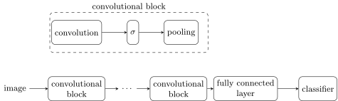
The standard scheme of a convolutional network (schematic): "convolution — nonlinearity — pooling" blocks are repeated, reducing the size of the image and increasing the number of channels; on top of them are fully connected layers and a classifier (Yann LeCun et al., 1995).
AlexNet: a convolutional network learns to extract features
Let us look at how one of the classical convolutional networks is arranged — the very network AlexNet that in 2012 brought about the revolution in computer vision. Depending on how you count, it has seven or eight layers. The original image is, to be concrete, in size, and 3 is the dimension of the vector that sits in each pixel. is the size of the neighbourhood of the first convolution. Why 96 here? These are 96 different convolutions that we compute at each pixel. Then layer by layer, thanks to pooling, the size decreases — you can trace it: 55, 27, 13 and so on — and at the end we in effect get a picture of pixel. We reduce the size until we have pulled the image into a point, but all the while we increase the dimension of the vector that sits in each pixel: 256 and so on, up to 4096. This means that, by putting several convolutions one after another, we have pulled the image into one pixel but increased the dimension of the vector, that is, in the end we have obtained a vectorisation of the image: we have generated 4096 features of the image. The whole convolutional part of the network carries out the vectorisation of the image. After that you can do whatever you want with this vector: for example, put two or three fully connected layers and get a neural network for recognising objects in an image. It consists of two large pieces: the convolutional layers, which in essence performed the vectorisation, and a multilayer fully connected network that carries out recognition on these vectors.
Remark (The higher the layer, the larger and more complex the image elements it recognises). Conv 1: edges and blobs (edge + blob); Conv 3: textures (texture); Conv 5: object parts (object parts); Fc8: object classes (object classes).
Krizhevsky A., Sutskever I., Hinton G. ImageNet classification with deep convolutional neural networks. 2012.
The pictures on the slide are an attempt to interpret what each layer does. We go through images, optimise them in a special way and find ones that lead to a strong response in the given layer of the neural network; having found the images that give a strong response, we get an answer to the question of what the given layer recognises. It turns out that the first layers recognise some gradient transitions: some edges, transitions, black-and-white in places, coloured in others. Why coloured? Because the convolutions in the first layer are done over RGB vectors, and some convolutions may use only one colour, while others use some aggregation of colours: if you add up all the colours, you get a black-and-white analogue of the image in grey. Further on, going layer by layer, pooling reduces the size of the picture, which means that each next layer sees larger image elements than the previous ones saw. After the gradients, textures start to be recognised; the next, higher layers recognise more complex elements, not yet interpretable, and the further we go, the more interpretable the pieces of image we see: the noses and eyes of dogs, elements of objects that were in the original sample. In the last layer a vector representation of the image is formed, and if we want to recognise, say, 20 thousand different objects, the information about these twenty thousand objects ends up encoded in a vector of dimension four thousand. This vector will be enough to tell whether each of these twenty thousand objects is present in the given image.
Remark (RGB and convolutions). A question: is the convolution done over each of the R, G, B matrices separately?
No: we consider that an RGB vector of dimension 3 has arrived in each pixel, and then we can do anything with these vectors — build convolutions that work only with individual colours or with all of them together, that do averaging.
Remark (How the layer pictures were obtained). A question: how was the picture under AlexNet obtained?
The original images from the ImageNet dataset are cut into fragments so that they can be identified at the output of the neurons of the given layer. Studying, for example, the first convolution layer, we look at which image fragments make the neurons of this layer give a large output value, that is, respond to them specifically, and we cut out the fragments that gave the largest responses. The fragments can be cut straight from the original pictures, or images can be generated: the slide has both generated fragments and fragments from the real dataset. There are publications on how these experiments were done: their aim was not to build a neural network but to explain why and how a convolutional network and each of its layers work.
ImageNet and the deep learning revolution
Definition (ImageNet, a large sample of labelled images). 2.5 years of labelling (2008/07–2010/04); 14 197 122 images; 21 841 object classes; 3 labellings of each image.
Li Fei-Fei et al. ImageNet: A large-scale hierarchical image database. 2009. Li Fei-Fei et al. Construction and analysis of a large scale image ontology. 2009.
The large collection of images is called ImageNet; the first publications on it date from 2009, and then the ImageNet competition was launched. How to count errors in ImageNet is a separate and not very simple question; we will not go into it now. The classical computer vision algorithms that existed in 2010–2011 gave about 25% errors. And then the deep neural network AlexNet appeared — Geoffrey Hinton with his graduate students. The most important thing that was invented, besides several heuristics that worked well together, was an implementation on graphics cards: it made it possible to experiment and actually train this network of eight levels with a huge number of parameters. After that, this competition was led exclusively by deep neural architectures, until in 2015 another epoch-making model appeared — ResNet, which made it possible to increase the number of layers sharply.
Remark (Deep convolutional networks for image classification). The competition started in 2009; the human error level of 5% was passed in 2015. The convolutional network AlexNet: ReLU + dropout; 60 million parameters; enlarging the sample; choosing the layer sizes; GPU.
Which heuristics worked together? First, ReLU was used; second, dropout; third, augmentation: distorted versions of the original images were generated — shifted, scaled, with some changes in colours. This increased the size of the sample, and at the same time the network learned to be invariant under certain transformations; augmentation is a good trick for training neural networks on images. Then there were experiments with architectures and with the number of parameters, and in the end they settled on a network with 60 million parameters, most of them in the fully connected layers. One has to understand that convolutional neurons are very sparse: they look only at the neighbourhood of the given pixel. If a convolutional neuron has a neighbourhood, only 9 coefficients are non-zero, and all the others are simply cut out of the network: they are not even computed and take no part in the backpropagation algorithm — we know where the zeros are, there is no need to go through them. And the use of graphics cards made it possible to compute orders of magnitude faster and therefore to run a large number of experiments to choose the architecture and all kinds of parameters: all the sizes of the convolution and pooling layers were chosen as a result of a large number of experiments.
Remark (Convolution layers and training tricks). A question from the chat: how are ordinary normalisation and dropout used in convolution layers?
Convolution layers do not differ in principle from ordinary ones, except in two things. First: we agreed that in each neuron some connections are absent — we zeroed some coefficients. This cannot affect anything, neither backpropagation (we simply exclude the zero coefficients from the loops) nor the possibility of applying any other heuristics: imagine a fully connected network in which you know for certain that some coefficients are zero — that gets in the way of nothing. Second: at each pixel you compute not one convolution but many — this too affects nothing. Look again at the AlexNet picture. The little cube on it is a symbolic depiction of the topology: each neuron that sits in it is in fact linked to some region of the image, it has a centre tied to a particular pixel. This cube is nothing other than a huge number of neurons, : each neuron knows which particular neurons of the previous layer it takes, and if you trace them back to the very beginning, they are tied to particular pixels of the image. And 256 means that at each point of the image you compute 256 different convolutions and train them differently: some convolutions take only the red colour, some the grey image, some smooth in different ways, one takes the nearest pixels with a large weight, another the diagonal ones. Each convolution is a filter over the image. Unroll the cube into a vector, and you get neurons — in terms of a fully connected network you have simply zeroed some coefficients. So all the tricks applicable to fully connected networks are applicable to convolutional ones too.
As for the question of why batch normalisation and dropout are not used together — I have heard that somewhere too, but I have not looked in detail into why they interfere with each other; I am not ready to give references offhand.
ResNet: the residual neural network
Another epoch-making algorithm is ResNet, the residual neural network. The idea is actually very simple. Imagine that you carry out a transformation with a layer of a neural network: you transform the input into the output. The output can simply be the identity transformation — pass the input on to the output. Formally this increases the number of layers, but clearly it is a cheat: you train nothing in this layer. The question is: can this trivial idea, that what was received at the input can simply be fed to the output, be corrected somehow? The idea arises of adding the outputs of previous layers to the output of the current layer.
Definition (ResNet: the residual neural network (Residual NN)). A skip connection of layer with a preceding layer :
Layer computes not a new vector representation but its increment .
- Increments are more stable convergence improves.
- It becomes possible to increase the number of layers.
- A generalisation is Highway Networks:
Kaiming He, Xiangyu Zhang, Shaoqing Ren, Jian Sun. Deep Residual Learning for Image Recognition. 2015. R. K. Srivastava, K. Greff, J. Schmidhuber. Highway Networks. 2015.
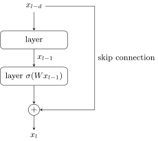
A skip connection in a residual network (schematic, ): the output of layer is added to the output of layer , bypassing the intermediate layers, so that the layers learn to compute only the increment.
In general form this skip connection, or shortcut connection, looks like a sum: the output of a layer is now not only an ordinary neuron (an activation function — not necessarily a sigmoid; residual networks most often use ReLU — of a linear combination), but the output of some previous layer is added to it as well, and not necessarily but : several layers can be skipped. is the layer number, the number of layers skipped; in the picture two layers are skipped, usually one is skipped, but it can be more. The same backpropagation is easily written out for such a transformation too, but stability improves: thanks to this untrainable identity transformation, the vectors obtained in previous layers are used directly. And the main effect of this type of network is that the number of layers can be increased with impunity. Note how sharply the number of layers grew: before, people could not build neural networks deeper than a couple of dozen layers, beyond that there were stability problems, while ResNet made it possible to build 150 layers.
In the same year, 2015, a generalisation appeared — the highway network, a slightly more complex formula. One more neuron is built at the side, called the transform gate, with an activation function that gives values from 0 to 1. Such normalisation lets us say: use the output of the current neuron with this weight, and the identity input from the previous layer with weight one minus the transform gate. The identity part means you simply carry over the vector you had before, and the transform means you add some transformation to it.
Convolutional networks for speech, texts and games
All these tricks together start to work very strongly, and the discovery of deep neural networks for computer vision is connected precisely with understanding in which combination all these heuristics have to be taken for them to really give a good result. Once it was understood how to deal well with images, the question arose: for what other complex input data can deep neural architectures be used?
Example (Recognising speech signals). Consecutive fragments of the signal are represented by vectors of the spectral decomposition.
Qirong Mao, Ming Dong, Zhengwei Huang, Yongzhao Zhan. Learning salient features for speech emotion recognition using convolutional neural networks. 2014.
Speech recognition is also in effect an image, because a sound signal can be represented as an image: one of its dimensions is time and the other is wavelength. You have done a fast Fourier transform and unrolled a one-dimensional signal into an image. Then you only have to stipulate that the windows, which in images were small neighbourhoods, are here small in time but are usually taken in full over the wavelengths. Then convolutions — and with very similar neural architectures one can recognise signals, speech and so on.
Example (Classifying sentences in a text). Consecutive words in a text are represented by vectors using vector representations (word2vec and others).
Yoon Kim. Convolutional neural networks for sentence classification. 2014. Yann N. Dauphin et al. Language modeling with gated convolutional networks. 2017.
The next variant is text. It would seem an object of a different nature, not like an image. But if you learn to represent words by vectors (we will talk about the vectorisation of words in the coming lectures), then each word is a vector and a text is a sequence of words, in effect an analogue of a time series, and you get something very similar to an image or to a sound signal. Convolutional neural networks are indeed used to solve problems on texts — classification and many others; we will talk about this during the semester.
Example (Decision making in logical games). David Silver et al. (DeepMind). Mastering the game of Go without human knowledge. 2017.
Another well-known application is an algorithm that can play Go. I only give the reference and will not go deep, but the idea is also very simple: a convolutional neural network is built on a principle very similar to images, and the last layers are again fully connected.
Remark (A convolutional network is a vectorisation of objects with a given topology). The idea works in many applications where you originally have objects with some complex structure. The main thing is that some topology should be defined, so that you know which elements of these objects are close to each other. On images you defined a neighbourhood — and if you have some definition of a neighbourhood, you can do a convolution over it, and then an analogue of pooling. Regardless of whether you have images or objects of another nature, if there is a notion of a neighbourhood on their elements, you can arrange the same vectorisation: layer by layer simplify the structure, pull it into one point, but at the same time layer by layer increase the dimension of the vector representation. In the end you get a vector of fairly high dimension at a point, and it should turn out to be enough to solve the problems you need. These can be graphs, they can be goodness knows what — the main thing is that there is a notion of a neighbourhood, and then one can figure out how to make a convolutional neural network.
Recurrent neural networks
Sequence processing problems
The next very important class of neural networks is recurrent neural networks; they are designed for processing sequences. Suppose we have a time series of vectors: at each moment there is an input vector — a description of some situation that we have to recognise or in which we have to make a forecast — and our goal is to form an output vector at each moment. For example, the input vector is information about the sales volumes of all goods in all the shops of a chain, and is a forecast of sales volumes for, say, the next two weeks. Here is an example of an applied problem where both the input vector and the output vector we want to forecast can be of fairly high dimension.
Definition (Sequence processing problems). Given: , a sequence of input vectors.
Find a model with parameter matrices , , that computes , the hidden state vector, , and , the output vector (in some applications ).
A two-layer network and its unfolded representation (unfolding):
The training criterion of a recurrent network:
where is the loss from the prediction at the moment .
What do we do to form from ? The sequence of pairs is our training sample. But besides that we assume that the process is so complex that it has some hidden state at each moment , and in the hidden state vector we will accumulate some information and pass it from one moment to the next. How is this idea implemented with a neural network? The vector is simply the output of the first neural layer: at the input we fed with the weight matrix , but we also fed to the input. This is what fundamentally distinguishes a recurrent network from everything we have studied before: the previous state, at the previous moment, is also fed to the input. This can be drawn as a scheme with feedback, but such a scheme does not show that it is precisely that was obtained, so a so-called unfolding is done and the network is drawn as a sequence over moments of time.
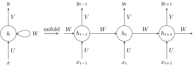
A recurrent network with hidden state and its representation unfolded in time (unfolding): the same matrices , , are applied at every moment.
One has to understand that all the matrices , and are the same at all moments. is what we use to form, from the hidden state, what we want to predict. Note that the formula for no longer contains the input. This means that the hidden state vector must contain all the information needed for the forecast: we have pushed the original information for moment , and the information accumulated over the whole history, which is in the vector , into the input of the neuron, and at the output we hope to get an informative vector that will let us form a forecast. In fact this network has two layers — here is the first layer, here the second — and the unfolding only shows graphically how the network works in time. We train three matrices, and when the neural network runs on a sequence they no longer change (during training, naturally, they do): step by step we apply one and the same neural network to all moments.
The loss function depends strongly on the applied problem. If you are solving a forecasting problem, you will most likely take the least squares method, the squared difference; if it is forecasting consumer demand or sales volumes, perhaps some other, asymmetric loss function. If the sequence is actually a text and you are going to tag its fragments or output some information for each word, the input can be the vector representations of the words, and the output the tags you mark these words with; then the loss function is the logarithm of the probability, because this is likelihood maximisation. In general it is a loss function that may be different at each moment and depends on , on the information at the moment and, naturally, on the parameters we are looking for.
Remark (Applications of recurrent neural networks). Time series forecasting; control of technological processes; classification of texts or their fragments; sentiment analysis of a document, sentences, words; machine translation; speech recognition; speech synthesis; synthesis of answers to questions, conversational intelligence; generation of image captions; generation of handwritten text; interpretation of the genome and other problems of bioinformatics.
Andrej Karpathy. The unreasonable effectiveness of recurrent neural networks. 2015.
Training recurrent networks: BPTT
How is this neural network to be trained? Here too I will not go deep into details: backpropagation is our everything. But there is a peculiarity here: each time, to compute the gradient accurately, all the past information has to be used. Strictly speaking, this can no longer be called a stochastic gradient, because we must always work through the sequence in time order: we cannot take and in arbitrary order, a strict "preceding — following" relation is given on them, and it is given in the very structure of the network. So we always run along the time series from left to right.
Definition (Training recurrent networks: Backpropagation Through Time (BPTT)). A special variant of error backpropagation:
To prevent vanishing and exploding gradients: .
D. Rumelhart, G. Hinton, R. Williams. Learning internal representations by error propagation. 1985.
Imagine that we have already run through a number of moments and now have to train the parameters , , by such a criterion. And, oh horror, the matrix is in all the terms: depends on through . In this formula the computational cost accumulates quadratically in time: note that here there is a sum over from 0 to over the whole history, and inside it a product. How is this dealt with? Usually it is assumed after all that there will be some decay and the oldest information is not really needed, so a time window is set, and one says: for training by backpropagation through time we will use not the whole history but only the previous 20, 50, 100 points — as many as the complexity of our data allows. And indeed, the loss functions can often be chosen so that old data have very little influence, and if we do not run so deep into the history, we will not lose very much.
The second problem is that we keep computing the derivatives , and a huge number of these partial derivatives are multiplied together. So in recurrent neural networks the question of how we solve the problem of exploding and vanishing gradients is very important: it is precisely here that this accumulation can happen. One has to use activation functions, and build the model, in such a way that these partial derivatives are, as far as possible, equal to one by construction; if we guarantee this, that is very good, and if they at least tend to one, that is also very good.
Long short-term memory networks (LSTM)
Now one of the most popular recurrent neural networks. It was in fact invented a very long time ago, in 1997, and for the following twenty years or so, research on this model, long short-term memory, was very sluggish: perhaps a few dozen papers a year. And suddenly, when the deep network revolution had already happened in computer vision, about two years later it turned out that LSTM networks are very effective for text analysis. Clearly, in 1997 there was not yet computing hardware powerful enough to train such networks well.
Definition (Long short-term memory networks (long short-term memory, LSTM)). The motivation of LSTM: the network must remember the history, that is, the context, for a long time; which context exactly, the network must learn by itself. is introduced, the vector of the network's long context at the moment .
where is the concatenation of vectors; is the sigmoid function; ; is the componentwise multiplication of vectors.
- The forget gate, with parameters , , decides which coordinates of the context vector to remember.
- The input gate, with parameters , , decides which coordinates of the context vector to update.
- The model of the new context, with parameters , , forms the vector with information about the new context.
- The new context vector is formed as a mixture of the old context vector with the gate and the new context vector with the gate ; there are no tunable parameters here.
- The output gate, with parameters , , decides which coordinates of the context vector go to the output; the output signal is formed from the context vector by the nonlinear transformation and the gate .
Hochreiter S., Schmidhuber J. Neural Computation, 9(8), 1997. Greff K., Schmidhuber J., 2015.
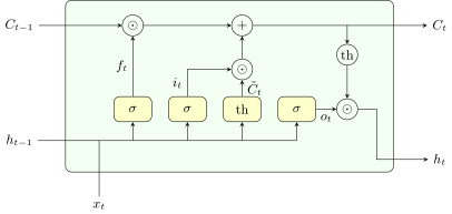
The scheme of an LSTM cell (ours): the context vector is passed along the top line; the forget gate damps the coordinates of componentwise, the input gate selects the coordinates of the candidate , and their sum gives ; the gate selects the coordinates of for the output . All four yellow blocks take the concatenation as input.
Architecturally LSTM really is non-trivial, and it answers the question of how to pass on information about the past. We accumulate a hidden state vector, but the idea is to split it into short-term and long-term memory: let us introduce one more state vector, the long-term memory, and build a neural architecture that will itself decide what to put into long-term memory and what not to. The dimension of this vector is a resource, and the network can spend these dimensions on keeping something important. The question is how to decide what is important and what is not, and the second question is how to encode this by neural means, since the only thing we can do is construct some neurons and stack them on each other. The result is this structure; let us work out why each block and each arrow is needed.
As usual in a recurrent network, there is an input vector and a hidden state vector passed on from the previous moment. A convenient notation often used in recurrent networks is the concatenation of two vectors: instead of two matrices and one can write one, if we consider that the concatenation is fed to the neuron's input; this is just shorthand. The first layer is the one we would have made in an ordinary recurrent network too, but we build several very similar neurons: one carries out a transformation of the information, and another, the forget gate, decides which coordinates of the vector are important to remember in our second state vector , the long-term memory. We will train the weight matrices, and they themselves will determine what we want to forget and what information to use for forecasts at each moment. We also introduce a model of the new state, which forms a vector of candidate values : at each moment we first compute what we would like to keep in long-term memory. Note that all these neurons essentially form the first layer: they take and as input, and their input is the same.
And now we start building the second layer, and it is unusual. The operation is the componentwise multiplication of vectors. and have a sigmoid activation function: its output is something from zero to one, which can be regarded as a weight coefficient. If you multiply and and the value in some coordinate of the vector is close to zero, you forget the corresponding coordinate of the vector . You combine two vectors — the previous state and the vector with information that could be put into long-term memory — and you specially train two gates, and , with separate neurons. The trainable gate indicates in which coordinates lies the information important to remember that was formed at the moment , and the gate , on the contrary, which information must be forgotten from the previous state.
Next, the output gate is formed — this is very similar to the second layer of an ordinary recurrent network. And finally, the output signal , which will be passed on to the next moment, is also a combination of the information formed at the output with the long-term information. On the one hand, is a vector that accumulates from one step to the next, and the information about the history is accumulated in it; on the other hand, this vector is used to impose a filtering transformation on the information that will be passed in to the next moment. If we count the layers: the first three lines are the first layer, is the second, the third, the fourth; and if is also formed on top of , there will be a fifth layer.
Remark (Why is needed). A question: why is needed?
If it were not there, you would simply pass the same information from one moment to the next, and the only thing you could do with it, thanks to the forget gate , is set some part of the coordinates to zero or close to zero. But you could add nothing to from the current iteration. is needed to form a candidate vector, some coordinates of which contain important information obtained precisely at this step — information that came from . Without it, information from the current step could not get into at all; it is a way of enriching the long-term memory vector with information from the current step.
Variants of LSTM and GRU networks
It seems that something here is overcomplicated, and one can see what could be worked on and done differently. The nature of the questions about LSTM is always the same: why is it done exactly this way, why not do it more simply, why not do it a little differently. There are many questions, and the answer to them is universal: do it that way and compare it with LSTM. That is what people do.
Definition (The LSTM variant with peepholes).
- All the gates "peep" at the context vector or .
- The number of model parameters increases.
- The number of layers increases, from three to four.
- A peephole need not be used for all the gates.
Gers F. A., Schmidhuber J. Recurrent Nets that Time and Count. 2000.
One direction is to enrich the architecture: feed the vector to the input of all three gates as well — forget, input and output — that is, let them look into the long-term memory. This naturally complicates the structure of the network: by increasing the input dimension we increase the dimensions of all three parameter matrices. It seems a useful idea, but it is a path towards complication.
Definition (A simplification of LSTM: Gated Recurrent Unit (GRU)).
- Only the state is used; the vector is not introduced.
- The update gate replaces the input and forget gates.
- The reset gate decides what part of the memory to carry forward from the previous step.
Cho K. et al. On the properties of neural machine translation: encoder-decoder approaches. 2014.
The other direction is, on the contrary, to simplify, and here is a very popular simplification: one layer fewer and one gate fewer — two gates are used instead of three — and the vector is not introduced. It is assumed that the vector , which passes information from the previous moment, contains everything needed, both short-term and long-term. For this, two gates suffice, called the update gate and the reset gate. Once you understand how LSTM works, it is very easy to understand how GRU works. In the first layer two vectors are formed, and , and then we act by analogy with what happened with the vector : the vector is formed from the of the previous iteration, to which we try to add information from the current step. decides in which coordinates we keep more of the information and in which we update it more. is the analogue of : the information we take from the current iteration and try to update the vector with. We try — but it may not work out: some of the coordinates we must still keep from the previous iterations, and that is exactly what the update gate is responsible for: it says what to update and what to keep. And is formed in effect as the second layer of a neural network and uses information from the previous moment and the current vector .
It turned out that in many practical problems, despite having fewer layers, fewer parameters and a simpler network overall, GRU often works no worse than LSTM. The problems that can arise from overcomplication are softened in GRU: there may be less overfitting, faster training, more stability. For some problems the expressive power of GRU may not be enough, and there LSTM will work better, but on the whole they are comparable in quality, and GRU is much simpler.
Conclusions
So, today two classes of neural networks: convolutional and recurrent. An important thing for understanding recurrent networks: although they are often drawn in unfolded form, do not let yourself be deceived — these are not layers. A recurrent network actually has two layers, and an LSTM four or five, depending on whether we build one more layer on top of . There is still an analogy with layers in that, to update the gradients, one has to go through the whole history each time, and there is a mass of mathematical tricks and devices for making backpropagation through time more stable. This material is too technical to present in lectures; it has to be looked up in publications. And what is when we process texts — how to turn words into vectors — is for the next lectures.
Remark (Summary).
- Convolutional networks: gradual vectorisation of complexly structured data, trained jointly with the main predictive model.
- Recurrent networks: trainable transformations of an input sequence into an output sequence (seq2seq).
- The tricks that made deep learning possible:
- advanced gradient methods speed up convergence;
- regularisation and dropout prevent overfitting;
- skip connections increase depth without overfitting;
- batch norm reduces computational errors;
- augmentation provides robustness to distortions;
- ReLU prevents vanishing and exploding gradients;
- convolutions and sparsification reduce the number of parameters.
- The transition from feature engineering to architecture engineering.
- Choosing the architecture and hyperparameters is still an art.
No comments yet
Be the first to share your thoughts.