August 30, 2026 · Lecture · LibreTimes
Machine Learning. Additional Lecture 1. The Theory of Overfitting
Contents
- What this lecture is about
- Reminder: the probability of overfitting
- Experiments with overfitting
- A monotone chain of algorithms
- How overfitting depends on the error matrix
- Overfitting of chains with different splitting
- Overfitting when choosing between two algorithms
- The combinatorial theory of overfitting
- The splitting–connectivity graph
- The generating and forbidden sets
- The splitting–connectivity upper bound
- Summary
What this lecture is about
The classical theory of generalisation — the Vapnik–Chervonenkis bound, capacity, structural risk minimisation, the "Occam's razor" bound — is set out in the first-semester lecture "Generalization Theory". Its main flaw is that the bounds are very loose. There are two reasons: the bound on the uniform deviation ignores the splitting of the family of algorithms, and Boole's inequality ignores the similarity of the algorithms. This lecture is about what happens when both effects are taken into account. First, experiments show how strongly splitting and similarity (connectivity) affect overfitting. Then a combinatorial theory is built: the splitting–connectivity graph of a family of algorithms, the generating and forbidden sets, and an upper bound on the probability of overfitting that takes both effects into account and in a special case turns into the Vapnik–Chervonenkis bound.
Reminder: the probability of overfitting
The first part of the slides for this lecture (pp. 3–20) repeats the problem setting and the classical theory; here we give only what will be needed later.
Definition (The error matrix and the probability of overfitting).
- is a finite general set of objects; is a split into a training and a test sample;
- is a finite set of algorithms; is the binary loss function;
- is the number of errors, is the error rate of on the sample ;
- is the learning method;
- the overfitting ;
- all splits are equally likely: .
The probability of overfitting:
Complete cross-validation:
The error matrix is the matrix with pairwise distinct columns: each algorithm is represented by its error vector. For a single algorithm with errors on the general set, the probability of overfitting is computed exactly:
where is the hypergeometric distribution function. For a family, the Vapnik–Chervonenkis bound is obtained in two steps — a bound on the uniform deviation and Boole's inequality:
The first step replaces the result of learning by the worst algorithm of the family and ignores the fact that the learning method picks algorithms only from the lower layers of the family by number of errors. This is the splitting effect. The second step adds up the probabilities of events as if they did not overlap, and ignores the fact that for similar algorithms the overfitting events almost coincide. This is the similarity effect, or connectivity effect.
Experiments with overfitting
A monotone chain of algorithms
How can the similarity of algorithms be taken into account, and not only splitting? The simplest model of a family of similar algorithms is a chain.
Definition (A chain of algorithms). A chain is generated by a continuous change of a parameter, for example by a threshold decision rule over a feature :
In a chain each next algorithm differs from the previous one on only one object.
Example (A chain of threshold rules: 2 classes, 6 objects, 7 threshold algorithms). The objects are ordered by the value of the feature ; the classes are : are of class , of class . The threshold stands before the object ; the rule assigns the objects to the right of the threshold to class . The error matrix:
| 1 | 0 | 0 | 0 | 0 | 0 | 0 | |
| 1 | 1 | 0 | 0 | 0 | 0 | 0 | |
| 0 | 0 | 0 | 1 | 1 | 1 | 1 | |
| 0 | 0 | 0 | 0 | 1 | 1 | 1 | |
| 1 | 1 | 1 | 1 | 1 | 0 | 0 | |
| 0 | 0 | 0 | 0 | 0 | 0 | 1 | |
| 3 | 2 | 1 | 2 | 3 | 2 | 3 |
A chain of threshold rules (slide): objects of two classes on the feature axis, the thresholds , and the number of errors of the rule with threshold .
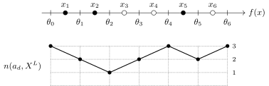
A chain of threshold rules: objects of two classes on the feature axis ( filled, unfilled), the thresholds , and the number of errors of the rule with threshold . Neighbouring rules differ on one object, and the number of errors changes by one.
Moving the threshold past one object changes the rule's answer on exactly that object, so neighbouring columns of the error matrix differ in one row, and the number of errors changes by one, in one direction or the other. Threshold rules over one feature, conjunctions of threshold conditions, linear classifiers under a continuous change of the weights — in all these families similar algorithms form such chains and their multidimensional generalisations.
How overfitting depends on the error matrix
Definition (An experiment with four error matrices). The upper bounds of VC theory depend only on the size of the error matrix, , and are therefore very loose.
The experiment: compare and CCV for four error matrices:
- the best algorithm is the same;
- there is or is not splitting — when each next algorithm makes one more error than the previous one;
- there is or is not connectivity — when each next algorithm differs from the previous one on only one object.
K. V. Vorontsov. Splitting and similarity phenomena in the sets of classifiers and their effect on the probability of overfitting. PRIA, 2009.
The four matrices are built to differ only in these two properties. With splitting and connectivity: a monotone chain, each next error vector obtained from the previous one by adding one error. Connectivity without splitting: a chain in which the error on one object is moved to another, and the number of errors does not grow. Splitting without connectivity: vectors with a growing number of errors, but random, unlike one another. Neither: random vectors with the same number of errors. The learning method in all cases is empirical risk minimisation; the probability of overfitting and CCV are estimated by the Monte Carlo method over random splits.
The probability of overfitting as a function of the number of algorithms (slide), , , , Monte Carlo splits. The colour of a curve is the colour of the matrix's frame: red — splitting and connectivity, green — connectivity only, blue — splitting only, magenta — neither.
Remark (Conclusions from the experiment).
- Connectivity slows the growth of the curve .
- Splitting lowers the level of the horizontal asymptote.
- Huge families with splitting and connectivity may hardly overfit at all.
- The VC bound linearly majorises the worst of these curves.
Without either effect the probability of overfitting grows quickly with the number of algorithms and is already close to one at a hundred algorithms. Connectivity without splitting slows this growth: the curve grows almost linearly and slowly. Splitting without connectivity stops the growth: from about fifteen algorithms on, the curve reaches a horizontal asymptote, because algorithms from the upper layers are never chosen. Both effects together give an asymptote of about after only a few algorithms. The Vapnik–Chervonenkis bound grows in proportion to and does not distinguish these four cases.
The complete cross-validation estimate as a function of the number of algorithms (slide), , , . For each matrix there are two curves: above, ; below, .
Remark (Conclusions for CCV).
- Without splitting and connectivity even 10 algorithms can overfit badly.
- Without taking the splitting and connectivity effects into account, exact bounds on the probability of overfitting cannot be obtained.
The error rate of the best algorithm on the general sample is the same in all four cases, . The gap between the error rates on test and in training is precisely overfitting on average. With splitting and connectivity it is small: the test error rate is about . Without either effect the training error rate falls to , and the test error rate grows almost to : the learning method finds in the family an algorithm that happens to fit the training sample well. Without splitting the gap appears already within the first ten algorithms.
Overfitting of chains with different splitting
A chain can be arranged in different ways: the number of errors along it may grow monotonically from the best algorithm, or it may have several local minima, or stay almost constant for a long time.
Example (Overfitting of chains with different splitting). Experimental conditions: , , , random Monte Carlo splits.
For six chains with different profiles of the error rate along the chain, the mean error rate of ERM in training and on test was computed: a monotone chain from the best algorithm; a V-shaped chain with one minimum in the middle; a chain with three minima; a chain that reaches a noisy plateau; a plateau with one dip; a chain along which the error rate is almost constant.
Sh. Kh. Ishkina. Combinatorial bounds of overfitting for threshold decision rules. 2018 (in Russian).
The weaker the splitting of a chain, the greater the overfitting. For the monotone chain the error rates of ERM in training and on test almost coincide: about and . For the V-shaped chain the gap is larger, for the chain with three equal minima larger still. The chain that overfits most is the one along which the error rate is everywhere close to the minimum: about in training and about on test. Many almost equally good algorithms is exactly what the absence of splitting means: the learning method has many candidates, and one of them will by chance fit the training sample better.
Overfitting when choosing between two algorithms
The simplest case in which both effects are already visible is a family of two algorithms.
Definition (A family of two algorithms). ; suppose that for the algorithms the numbers are known:
The similarity of the error vectors is measured by the Hamming distance:
The splitting is measured by the difference in the number of errors:
Experimental conditions: , , , the Monte Carlo method over random splits.
The objects fall into four groups: on objects both algorithms err, on only , on only , on neither. The error vectors differ on objects, and the numbers of errors by .
The similarity and splitting effects for a pair of algorithms (slide): the probability of overfitting as a function of the Hamming distance for splitting ; thin lines are Monte Carlo estimates, thick lines their smoothing.
Remark (Conclusions for a pair of algorithms).
- Overfitting occurs even when choosing between two algorithms.
- The more similar they are, the less the overfitting.
- The greater the splitting, the less the overfitting.
If two algorithms coincide almost everywhere ( is small), choosing between them changes almost nothing, and the probability of overfitting is close to that for a single algorithm. As grows it grows, and with equal numbers of errors () it approaches . If, however, one algorithm is noticeably worse than the other (), the learning method almost always chooses the better one, and the probability of overfitting stays half as high for any .
For two algorithms the probability of overfitting can be computed exactly.
Theorem (On the probability of overfitting). If and the method minimises the empirical risk (the number of errors in training), then for any
Proof. Let , , objects from the first three groups fall into the training sample; the probability of this is the multivariate hypergeometric distribution, the first factor. In training makes errors and makes . The empirical risk minimisation method chooses if , and otherwise (in a tie, ). The chosen algorithm, with errors on and errors in training, overfits if , that is, , as in the case of a single algorithm.
The combinatorial theory of overfitting
The splitting–connectivity graph
The experiments show that overfitting is determined not by the size of the family but by how its error vectors are arranged: how far they are split by the number of errors and how far they are connected by the similarity relation. This structure is described by a graph.
Definition (The splitting–connectivity graph of a set of algorithms). Define binary relations on the set of algorithms :
- the partial order : for all ;
- precedence : and .
The splitting–connectivity graph : is the set of pairwise distinct error vectors; .
Properties of the splitting–connectivity graph:
- it is a subgraph of the Hasse diagram of the order relation on ;
- each edge has an edge object such that , ;
- the graph is multipartite with layers , .
An algorithm is no worse than in the sense of the order if errs only where errs too. Precedence means that is obtained from by adding exactly one error; the object of that error is the edge object . Edges go only between neighbouring layers, from layer to layer , so the graph is multipartite. The vertical structure of the graph is the splitting, and the edges are the connectivity: similar algorithms are joined.
Example (A family of linear classifiers). For a sample of ten points on the plane, linear classifiers generate in layer 0 one error vector with no errors, in layer 1 five vectors with one error, in layer 2 eight vectors with two errors, and so on (the error matrix of this sample is given in the first-semester lecture "Generalization Theory"). The splitting–connectivity graph is diamond-shaped: the layers first widen and then, towards vectors with many errors, narrow.
A family of linear classifiers (slide): a sample of ten points of two classes with several separating lines, and the splitting–connectivity graph of the family; the layers are the number of errors from 0 to 10, with layers 0, 1, 2 marked.
Example (A monotone chain). A monotone chain of algorithms: .
Example: a one-dimensional threshold classifier ; 2 classes , 6 objects: are of class , of class to the right of them; the thresholds move to the right past . The error matrix:
| 0 | 1 | 1 | 1 | |
| 0 | 0 | 1 | 1 | |
| 0 | 0 | 0 | 1 | |
| 0 | 0 | 0 | 0 | |
| 0 | 0 | 0 | 0 | |
| 0 | 0 | 0 | 0 |
The splitting–connectivity graph of a monotone chain (slide).
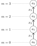
The splitting–connectivity graph of a monotone chain: one vertex in each layer ; the edge is labelled by the edge object .
Example (A two-dimensional net of classifiers). Example: a two-dimensional linear classifier, 2 classes , 6 objects. The lines are obtained by shifting and rotating the separating line: is the number of errors on the objects of one class (), on the objects of the other (). The error matrix:
| 0 | 1 | 0 | 1 | 1 | 0 | 1 | 1 | 1 | 0 | |
| 0 | 0 | 1 | 0 | 1 | 1 | 0 | 1 | 1 | 1 | |
| 0 | 0 | 0 | 1 | 0 | 0 | 1 | 1 | 0 | 0 | |
| 0 | 0 | 0 | 0 | 0 | 1 | 0 | 0 | 1 | 1 | |
| 0 | 0 | 0 | 0 | 0 | 0 | 1 | 0 | 0 | 0 | |
| 0 | 0 | 0 | 0 | 0 | 0 | 0 | 0 | 0 | 1 |
The splitting–connectivity graph of a two-dimensional net of classifiers (slide).
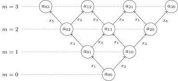
The splitting–connectivity graph of a two-dimensional net of classifiers: the vertex lies in layer ; each edge is labelled by its edge object, the one on which the successor algorithm makes an extra error.
A monotone chain is a one-dimensional structure: each algorithm is obtained from the previous one by adding one error. A two-dimensional net arises when the classifier has two degrees of freedom: the separating line can be moved so that it adds errors on the objects of one class, or so that it adds them on the objects of the other. Then two edges leave every vertex except the extreme ones. For linear classifiers in a space of higher dimension the graph is more complicated, but the edges still join similar error vectors, and the layers still split the family by the number of errors.
The generating and forbidden sets
To obtain a bound on the probability of overfitting, we need to understand for which splits the learning method chooses a given algorithm. For this, two characteristics of a vertex of the graph are introduced.
Definition (The generating set and upper connectivity). The upper connectivity of an algorithm is the number of all edges leaving the vertex in the splitting–connectivity graph:
is called the generating set of the algorithm .
Definition (The forbidden set and inferiority). The inferiority of an algorithm is the number of distinct edge objects on all paths leading into :
is called the forbidden set of the algorithm .
The generating set consists of the objects such that adding an error on any one of them gives a neighbouring, slightly worse algorithm. The forbidden set consists of the objects on which errs while some better algorithm does not. If even one such object falls into the training sample, turns out better than in training, and the empirical risk minimisation method will not choose . Hence the name: these objects "forbid" the choice of .
Definition (The splitting and connectivity characteristics of an algorithm).
- upper connectivity ;
- lower connectivity ;
- inferiority ;
- the number of errors .
Proposition. .
Every object of a lower edge , , belongs to the forbidden set, which gives the first inequality. Every object of the forbidden set is an error of the algorithm , which gives the second. Upper and lower connectivity and inferiority measure different things: is how many similar, slightly worse neighbours the algorithm has; is how much better algorithms "screen" .
Example: a fragment of a two-dimensional net of algorithms (slide). For the vertex in layer : (green edges upward), (red edges downward), .
The splitting–connectivity upper bound
Definition (A monotone learning method). An empirical risk minimisation method is monotone if
where is a strictly monotone function of the error vector of on the sample : for any and , if for all and the error vectors of and on differ, then ; and if they coincide on , then .
Example. The function is strictly monotone.
Theorem (The splitting–connectivity bound). For any monotone method , any , and
where , , .
K. V. Vorontsov, A. A. Ivahnenko, I. M. Reshetnyak. Generalization bound based on the splitting and connectivity graph of the set of classifiers. 2010.
Proof.
-
From build a monotone pessimistic method that maximises the overfitting:
Then is an upper bound.
-
If , then because is pessimistic, and because is monotone.
-
Therefore
-
By the law of total probability:
Let us explain steps 2 and 4. Suppose the pessimistic method has chosen . If some object of the generating set were in the test sample, the neighbouring algorithm would have as many errors in training as , that is, it too would be among the best, while erring more on test; the pessimistic method would have chosen . So all the objects of the generating set are in training. If some object of the forbidden set were in training, there would be an algorithm with a smaller value of in training, and would not have been chosen. So all the objects of the forbidden set are in the test sample. The probability that given objects fall into training and given objects into test equals the share of such splits: the remaining training objects are chosen from the remaining ones. Under this condition the algorithm makes no error on any object of and errs on all objects of ; among the remaining objects it has errors, and overfitting is again described by the hypergeometric function, but on a smaller set.
Remark (Properties of the splitting–connectivity upper bound).
-
For it is the hypergeometric distribution function:
-
For and it is the Vapnik–Chervonenkis bound:
-
The contribution of an algorithm decreases exponentially:
- in connected families overfit less;
- in only the lower layers contribute to .
-
The probability of obtaining an algorithm as the result of learning:
-
The bound is exact (becomes an equality) for multidimensional monotone nets of algorithms.
For the factor is approximately : each object of the generating set falls into training with probability about one half, and each object of the forbidden set into test. So an algorithm with large connectivity or large inferiority contributes almost nothing to the bound. Inferiority grows with the layer number, and the sum is in effect taken over a few lower layers of the graph. This is the quantitative expression of the splitting and similarity effects that the Vapnik–Chervonenkis bound ignores: with , that is, if neither is taken into account, the bound turns into it.
Summary
- Without splitting and connectivity, overfitting sets in already at a few dozen algorithms.
- Splitting and connectivity greatly reduce overfitting and can compensate for the effect of dimensionality.
- In practice families as a rule have them.
- A scheme for applying bounds on the probability of overfitting:
- estimate over a few lower layers;
- by inversion, estimate through ;
- use the estimate as an external criterion or a regulariser for choosing the model structure.
- The looseness of the bounds on can lead to underestimating the complexity of models (oversimplifying them) in this scheme.
- It is more practical to use cross-validation estimates.
- Tight upper bounds on overfitting are derived in COLT (Computational Learning Theory).
The combinatorial theory explains why complex models in practice overfit much less than the Vapnik–Chervonenkis theory predicts. A huge number of algorithms in a family is not in itself dangerous: what is dangerous is many equally good algorithms unlike one another. Real families — threshold rules, conjunctions, linear classifiers — are split and connected, and their probability of overfitting is determined by a few lower layers of the splitting–connectivity graph. The bounds of this theory can be used for model selection in the same way as the Vapnik–Chervonenkis bound in structural risk minimisation, but they too remain upper bounds. So in practice cross-validation is the more reliable way to choose a model.
No comments yet
Be the first to share your thoughts.