August 30, 2026 · Lecture · LibreTimes
Machine Learning 2. Lecture 8. Association Rule Mining
Contents
- What this lecture is about
- The problem setting
- Definitions and notation
- Market basket analysis
- Association rules are logical regularities
- The APriori algorithm
- Anti-monotonicity and the two stages
- Stage 1: finding frequent itemsets
- Stage 2: extracting association rules
- Drawbacks of APriori and modifications
- The FP-growth algorithm
- Stage 1: building the prefix FP-tree
- Properties of the FP-tree
- The support of an arbitrary itemset from the FP-tree
- The FP-growth algorithm
- Stage 2: recursive search for frequent itemsets
- The conditional FP-tree
- The efficiency of FP-growth
- Summary
- Seminar
What this lecture is about
Today's lecture is devoted to methods of association rule mining. It is no accident that it comes right after the logical classification algorithms: there is a strong analogy between mining association rules and searching for logical regularities — conjunctions — as we will see in a moment. But the main difference is that association rule mining is a method of unsupervised learning.
The plan is this: first I will give the problem setting, then a simple algorithm, and then a cool algorithm that is really used in practice. In general, today's lecture stands out somewhat in the whole course: it will be in the spirit of a course on data structures and algorithms. Its main topic is the FP-growth algorithm: we will work out how to implement computationally efficient association rule mining properly.
The problem setting
Definitions and notation
Definition (A frequent itemset). is the object space; is the training sample; , , are binary features (items).
Each subset corresponds to the conjunction
If , then "the features from occur together in ".
The frequency of occurrence (support) of the itemset in the sample :
If , then "the itemset is frequent" (frequent itemset). The parameter is the minimum support, MinSupp.
As usual, we have a training sample, and the objects are given by binary features — this is important. To each subset of features one can assign the conjunction of these features. There is a small liberty in notation here: by I will denote both the subset of features and the function of an object that is the conjunction of these features. These are two quite different mathematical objects, but there is a one-to-one correspondence between them, so they are denoted by one letter. I think you will quickly get used to this, and there will be no misunderstandings.
If the conjunction returns one, this means that all the features from the itemset have the value one on the given object , and we will say that the features of this itemset occur together in the object . In general we will say that a feature occurs in an object if .
Next, let us look at the set of objects on which the features from occur together, and agree to denote the frequency of occurrence of in the sample by : it is the share of sample objects on which the features from occur together. One can put it this way: in the object–feature matrix a submatrix is picked out that consists entirely of ones. On the feature side we picked out the columns from , and on the object side the rows that have only ones on this subset of features. The share of objects of this submatrix we call the frequency of occurrence, or support, of the set of features in the sample. If this support is large enough, we call a frequent itemset. Why this terminology took hold, why the columns of this matrix are now called not features but "items", we will understand in a moment from examples of practical problems.
Definition (An association rule). An association rule is a pair of disjoint itemsets such that:
- the itemsets and frequently occur together:
- if occurs, then also frequently occurs:
is the confidence of the rule. The parameter is the minimum support, MinSupp; the parameter is the minimum confidence, MinConf.
Here is the key definition we will need today: what an association rule is. It is two subsets of features, between which one usually puts an implication: from follows . It is a pair of disjoint itemsets such that, first, their union is a frequent itemset, that is, the support of exceeds some threshold ; this threshold is called MinSupp, the minimum support. In other words, and frequently occur together, they form a frequent itemset. The second condition: if occurs, then also occurs frequently. This is written by a formula very similar to the formula of conditional probability: among the objects where occurs, we pick out the objects where occurs together with , and their share turns out high enough — above a confidence threshold called MinConf. These two conditions, MinSupp and MinConf, are denoted exactly so in the literature; this too has taken hold. They define the pair of itemsets that forms a rule: if we observe the set of features in an object, then with high probability the set of features will be observed too. And "with high probability" means that the conditional probability exceeds MinConf.
Market basket analysis
Example (The classic example: market basket analysis). Market basket analysis [1993]: the features are goods (items); the objects are receipts (transactions). means that the -th receipt paid for the item .
Example: "if bread is bought, then milk will also be bought with probability ; and both items are bought together with probability ".
Possible applications:
- optimising the placement of goods on the shelves;
- forming personal recommendations;
- planning advertising campaigns (promotions);
- managing prices and the product range more effectively.
Where did such a problem come from? In the nineties, when data mining became popular, one of the problems that became very popular was market basket analysis. The problem is this. There is a huge supermarket, customers buy some goods in it, and by a basket we mean the set of goods a person has bought, at the exit from the shop. We have a set of receipts: each receipt is a transaction, one customer bought these goods together. The rows of our object–feature matrix are now in effect receipts, and the columns are goods. Clearly there can be a huge number of receipts, millions, and a large supermarket has some hundreds of thousands of goods. We really do have very big data on how people buy particular goods together.
And one can notice that there are regularities like this: people often take certain goods together. For example, if a person bought bread, then with high probability they will also buy milk; if they bought sausages, they will buy ketchup; if they bought beer, they will buy crisps. This is not an exact condition but a probabilistic one: an "if — then" rule that holds with some probability. That probability is exactly what confidence gives. Our task is to find all such cases where people buy something together, which goods are bought with each other.
A mass of applications can be found for this, to improve the sales of goods. One can optimise the placement of goods on the shelves. One can form personal recommendations: if we have an online shop, we can already make offers to a regular customer based on what is often taken together with the goods they have just put into the basket. Planning promotions, managing prices, the product range and so on.
So such a problem arose, and a story even wanders through many textbooks on data mining: supposedly in one large supermarket chain, when such a system was introduced, they discovered a regularity that on Friday evenings nappies were for some reason very often bought together with beer. And when the shelves with nappies and the shelves with beer were placed next to each other, this supposedly brought such profit across the whole chain that it almost paid for introducing the whole system. But in fact this story is made up: if it really worked, it would be in many supermarkets. And my attempt to find, through search engines, a photograph of a rack where beer and nappies stand side by side was not crowned with success. Yet there are hundreds of retellings of this story in various business courses on data mining. So it is more of an anecdote.
Association rules are logical regularities
Definition (A logical regularity and an association rule). A predicate is a logical regularity of the class if
where is the number of "" examples of the class and is the number of "" examples of the class .
For the rule "" take the target feature . Then
Conclusion: the differences between the two definitions are purely terminological.
Let us see that there is a deep analogy between these probabilistic rules and the notion of a logical regularity as we had it in the last lecture. Let me remind you: in the problem of association rule mining we had no classes; both subsets, and , we have to find and pick out in the original set of features. But if we had classes and had to solve a classification problem, we could define for the given class the share of its own objects that the given predicate picks out — it may be, among other things, a conjunction. The share of objects the rule picks out is nothing other than support: it coincides by definition. And if we impose the condition that among the objects the rule picks out, the share of its own must exceed some threshold, we get the same confidence. Here is the number of positive examples of the class and the number of negative examples of the class ; these are exactly the same definitions as in the last lecture.
The analogy shows that association rules and logical regularities are, on the whole, exactly the same thing; the difference is in terminology. Well, and the difference, of course, is that in a classification problem is the class, and we want to pick out the objects of one class , while in association rules, instead of the class , there is some subset of features, a conjunction, which also has to be found. That is, there is no ready class feature given in advance. But the conditions for finding regularities, support and confidence, are the same both in searching for informative conjunctions, rule induction, as in the last lecture, and in association rules.
The APriori algorithm
Anti-monotonicity and the two stages
Lemma (Anti-monotonicity of support). For the conjunction and any , implies : adding features to does not increase the support.
Corollaries:
- if is frequent, then all its subsets are frequent;
- if is not frequent, then all itemsets are not frequent either;
- for any .
Proof. If new features are added to a conjunction of binary features, the set of objects on which the conjunction returns one either stays the same or narrows. All three corollaries are one and the same statement in different formulations.
Now let us consider an important property that will let us build an efficient association rule mining algorithm, the property of anti-monotonicity. Take the conjunction of the features from the subset and add some number of features — make the itemset out of . The support can only decrease. Why? Because if we take more new features into a conjunction of binary features, the set of objects on which the conjunction returns one narrows — or stays the same.
Hence the corollaries — or rather, one and the same corollary in three different formulations. If is a frequent itemset, then all its subsets are frequent: their support is no smaller than the support of . If is not frequent, then all the itemsets that are its supersets are not frequent either: if occurs in too few objects of the sample, then by adding more features to we get an itemset that occurs even more rarely. So if we have built some itemset that is not frequent, it is useless to grow it: we will get no more frequent itemsets out of it. We will actively use this rule to add features to frequent itemsets gradually, getting new frequent itemsets from them. This will be the main point in the search for frequent itemsets.
By the way, if you look at the literature on association rule induction, most papers are actually about the problem of finding frequent itemsets; that is what they are called. It is the core of the association rule approach. Why? Because we will now split association rule mining into two stages.
Remark (The two stages of association rule mining).
- Finding frequent itemsets: repeated scanning of the transaction database.
- Extracting association rules: a simple efficient procedure in main memory.
The first stage, the hardest and most substantial, is precisely finding frequent itemsets. It is done by scanning the whole database of receipts, or transactions; this is big data, and it has to be scanned and all the frequent itemsets picked out. The second stage is building the association rules proper. When we have a frequent itemset, we can split it into two disjoint subsets and try to extract and from it. It will only remain to check whether the confidence condition holds: must follow from , that is, if is frequent, then is frequent too. This check of all possible splits of frequent itemsets into two subsets is a very fast and efficient algorithm. It is described once, implemented once, runs entirely in main memory, and there are no problems with it. So we will look at the second stage now too, and then forget about it as a closed, solved problem, and go on to the search for frequent itemsets.
Stage 1: finding frequent itemsets
Definition (The APriori algorithm (the main idea is breadth-first search)). Input: , the training sample; ; .
Output: , the list of association rules.
- the set of all frequent original features: ;
- for all :
- the set of all frequent itemsets of cardinality : ;
- if , exit the loop over ;
- ;
- for all , :
- .
Let us look at the algorithm most often mentioned in textbooks on data mining, but never used in practice, because in practice it is slow and inefficient. But it shows the main idea of association rule mining — how it is implemented in principle. This is the APriori algorithm.
At the input we have the training sample, a binary object–feature matrix — the features are called items here — and two thresholds, MinSupp and MinConf. At the output we must get a list of association rules, that is, pairs , for each of which two conditions hold: MinSupp — their union must be a frequent itemset, and MinConf — the association " follows from " must hold with a conditional probability exceeding MinConf.
As the first step we pick out all the frequent original features. Clearly a frequent itemset can be a conjunction only of features that are frequent themselves. If some item occurs rarely, it is simply useless to us, and we throw it out at once. At the very first step we build the set of features that are frequent, that is, satisfy the MinSupp condition.
The second step is a loop over from 2 to . Remember, is the number of features; it can be large, there can be hundreds of thousands. But in fact we will never get to this ; we will always stop much earlier, when we stop getting frequent itemsets. This will happen much earlier for one simple reason: one can hardly imagine a large number of people who put absolutely all the goods in the supermarket into their basket. There are a few goods in a basket, well 20, well 30, and such large baskets are unlikely to contain frequent itemsets. So there is no need to fear the here.
What do we do in this loop? The main step: from , that is, from the set of frequent itemsets of the previous iteration, we make . We take all the itemsets from and try to add features to them one at a time in all possible ways — but so that the MinSupp condition holds, that is, so that frequent itemsets result again. All the new frequent itemsets contain exactly one feature more. If you recall the lecture on feature selection, the group method of data handling — which is breadth-first search — there was exactly the same idea; in effect it is the same mechanism as in feature selection. But there we called it beam search, because it was a truncated breadth-first search, while here it is a complete breadth-first search, BFS.
Further, by the principle of anti-monotonicity, the support of the set of features decreases with each addition of features, and at some point none of the itemsets will be frequent any more: we have exhausted all the frequent itemsets, and has come out empty. Then we exit the loop. In fact this is the normal exit from the loop; it will always be exactly this, and not on reaching . That is it, we have found all the frequent itemsets. This really is very easy to do with breadth-first search.
Now it only remains to try to split each of these frequent itemsets into two disjoint parts, to divide it into a premise and a consequence, into and . This will be done by a recursive function, called here. It has three arguments. is the list of all the association rules we will build: first we set it to the empty set, and at the output we must get the result of our algorithm, the list of all association rules. Then we pass to this function all the conjunctions, that is, all the itemsets we have found in all the . It takes and splits it into and in all possible ways; how it does this we will work out on the next slide.
Stage 2: extracting association rules
Definition (Extracting association rules: the function AssocRules). A simple recursive algorithm that runs fast, as a rule entirely in main memory.
Function .
Input: , an association rule. Output: , the list of association rules.
- for all (to avoid repeating ):
- ; ;
- if , then
- add the association rule to the list ;
- if , then .
is the serial number of the feature in .
This is the second stage, building association rules from the frequent itemsets: we have found the frequent itemsets, and now we split them. At the input are , the list of all association rules, to which this function will add new rules, and and , the rule we have at this stage. Note that when AssocRules is called for the first time for a frequent itemset , the second part is the empty set.
Then the function recursively does the following simple work. It takes one feature at a time from , moves it into , and checks whether we have got an association rule. If we have, we enter it into the list and call AssocRules once more, where contains one feature fewer and exactly that same feature more. So at each step we will move one more feature from to . To do this in all possible ways, we loop over all the features from and try to move them to one at a time. And if after that — the from which we removed a feature — is still not a single element, one more feature can be removed from it, and we call the function AssocRules itself recursively. Note that the recursion is started only for rules that were found: if the rule did not pass the confidence threshold, then moving further features from to would only reduce it, since the numerator does not change, while the denominator for is, by anti-monotonicity, no smaller than .
So I have told you this algorithm. One small technical subtlety remains: what is this condition on the features in the loop? We go through not all the features, but only in increasing order of their serial numbers. Why is this done? To avoid repetitions, when we move from to first the first feature, then the second, and then try to move again — first the second, then the first, that is, in reverse order we arrange the same split of the set into two disjoint subsets. To prevent this, we always move features into in increasing order. And it does not matter how the numbering is arranged, the main thing is that there is some numbering at all: is the serial number of the feature in the whole set. This is a purely technical point, so that when splitting a finite set into all possible subsets we do not go through all the possible orders of the features we move into the second subset.
Let us look once more at the APriori algorithm — I have now told it completely. It consists of two parts: the first is finding frequent itemsets, the second is splitting all the frequent itemsets in all possible ways into a premise and a consequence to form association rules. In the first part we check only support, we use only MinSupp, the threshold , while in the second part, on the contrary, only MinConf: support is already ensured by the first part of the algorithm, and we check only the confidence condition.
Remark (A question: how does the condition on the numbers rule out repetitions?). Thanks to this condition, the features in will have strictly increasing numbers: by construction we guarantee that the features that have come into always go in increasing order of their numbers. It will not happen that we test the set of features in all possible variants — ; ; and so on. To avoid this superfluous work, we guarantee that each subset is formed only once. The order of the features in does not matter to us, and we agree that it should be the increasing order of the numbers these features had originally, and it does not matter at all what numbering that is.
— And are and different subsets?
Of course they are different: a subset of two elements and a subset of three elements are different subsets. But and are the same subset. We need subsets, not sequences, and so we remove the ambiguity in forming the subset by permuting its elements: of all the permutations we choose only one.
Drawbacks of APriori and modifications
The main drawback of this algorithm in fact lies in the first stage. The second stage is a very simple algorithm that raises no questions. But in the first stage questions are raised by such a seemingly harmless thing as repeatedly computing the support of itemsets — this very .
Let us estimate what is. Suppose we have a huge transaction database: the objects, the rows, are receipts, and the features, the columns, are the goods in the receipts. Computing for a subset makes us run through the whole database. And this whole database is most likely located on disk: it simply will not fit into any main memory, there may be terabytes. This was of course especially a problem a quarter of a century ago, when this problem appeared: main memory then was certainly not measured in gigabytes, as it is now. Imagine that the whole object–feature matrix is stored somehow on disk, and you need to compute this seemingly harmless quantity, the support of an arbitrary subset of features. You are forced to go to the database. And now estimate how many times you will compute this quantity for various subsets of features — and you will understand that if the data do not fit into main memory, you have no chance of computing it quickly.
Hence the idea: it would be great to devise a data storage scheme such that one could, once, in a linear pass over the transaction database, compute some compressed information about all the frequent itemsets, put this information into main memory, and then search for frequent itemsets by accessing only this compressed information. The whole question of an efficient implementation is how to build an efficient way of compressing the information about frequent itemsets so that it fits into main memory.
Remark (Modifications of association rule induction algorithms).
- More efficient data structures for fast search of frequent itemsets.
- Searching for rules on a random subsample of objects with lowered , then selecting rules on the full sample.
- Hierarchical algorithms that take the hierarchy of features into account (for example, a product tree).
- Taking time into account: incremental and decremental algorithms.
But before moving on to that, let us talk a little about what happens in practice with association rule mining, how these algorithms are generalised, whatever they are — APriori or more efficient ones. First, there are many different ways of solving this problem; we will now look at one of them, which is still considered the state of the art, although it was devised quite long ago. But there are alternative ways too. For example, search for frequent itemsets not over the whole database but over some relatively small random subsample, but lower the MinSupp and MinConf thresholds, find more rules than needed, and then simply recheck them once on the whole full transaction database — indeed in one pass. This can be done too, but it is not guaranteed that all the association rules according to the definition with MinSupp and MinConf will be found.
What else happens? Consider a real situation: you want to find the regularity that milk is often bought with bread. Clearly by bread we can mean quite different product positions in the shop. What is an item? Each kind of bread is a separate item; each way of packaging — for example, half a litre of milk and a litre of milk, although it may be one producer — is two different goods, two different items. It is quite clear that in this rule you do not care which bread exactly or which milk exactly, and you must find this regularity not at the low level of items but at higher levels of the product hierarchy. This hierarchy always exists: bread is an internal vertex of the tree, it splits into bread from different producers, then into bread in different packaging, and so on; the same applies to other goods. One has to find association rules involving not only the lowest, terminal items but also any internal vertices of this tree. That is, we build a conjunction out of disjunctions, as it were: at the lower level we can say that is one of 30 kinds of milk or one of 50 kinds of bread. Building such more complex constructions is actually not hard, on the contrary, it is simpler: you go down the hierarchy from the top and gradually find more and more specialised rules — first more general ones, at the level of product categories, and then at the level of the goods themselves.
Further, in this problem there are all kinds of incremental algorithms that can, for example, take today's transaction database, add this portion of data to the existing data, and rebuild the association rules. Probably not all the rules will change; most will remain even with the newly arrived information taken into account, but new ones may form. And on the other hand, data become outdated: by adding today to the data, we remove from them some day that was three months ago. So we move over the data with a sliding window, and it matters to us not only to add new portions of data but also to remove old ones. It turns out that both increment and decrement must be performed, and the association rules must be rebuilt as this happens.
The FP-growth algorithm
Well then, enough talk; let us move on to really interesting algorithms and the interesting mathematics used here. The idea will be this. We will build a data structure called the prefix tree of frequent itemsets, the FP-tree (FP stands for frequent pattern). By construction it will contain all the information about all the frequent itemsets, but it will be a structure that is easy to fit into main memory: it will be small. And most importantly, we will build this structure in one linear pass over the transaction database, and after that we will no longer access the database at all. Everything we want to know about frequent itemsets will be laid down in this structure, although in some non-trivial way: to get information about a frequent itemset, a specialised query to this structure is needed, and we will understand how it is arranged.
Stage 1: building the prefix FP-tree
Example (The prefix FP-tree). Order all the features by decreasing .
Each object is described by a word in the alphabet ; the FP-tree is an efficient way of storing the dictionary; the levels of the tree correspond to the features, in decreasing order of .
Example: , features ; with the features are not frequent.
| matrix, | words |
|---|---|
a - - d - f - | d a |
a - c d e - - | d c a e |
- b - d - - - | d b |
- b c d - - - | d b c |
- b c - - - - | b c |
a b - d - - - | d b a |
- b - d e - - | d b e |
- b c - e - g | b c e |
- - c d - f - | d c |
a b - d - - - | d b a |
First of all, let us work out how this structure is built. The first step: we order all the features by decreasing support, and those that do not pass the MinSupp criterion are simply discarded.
Let us turn straight to an example. Shown here is a matrix: the rows are receipts, the columns are goods; objects in the rows, features in the columns. I denote each item by a little letter: if the item occurred in the receipt, the letter stands there, and if it did not, a dash. For example, someone bought the items , and , and so on; we see how these goods were bought together. To be concrete, let us agree that in our example the support threshold is three objects, . We see at once that then the features and are not frequent: occurred only twice, only once. We cannot build any frequent itemsets involving these features, so we throw and out of consideration at once.
Next, let us agree on how to represent the rows of this matrix. Since the matrix is very sparse, it is convenient to regard the rows of this matrix not as binary vectors with a large number of zeros but as sequences of letters: the letters denote features. We also agree that we have sorted all the features by decreasing support. When we represent a sparse binary vector by a word made of letters, the first place will always be taken by the most frequent letter. One can see that the column is the most frequent, it occurs almost everywhere, so the letter will always stand in first place if it is present. From we get : we threw out because it does not have the support. The next word, , turns into after reordering. Here are these words, and in each word the letters are ordered by decreasing support: .
Next we will take all the rows of this matrix in turn and pack them into a very efficient data structure — that very prefix tree. How is it arranged? First, the number of levels of this tree equals the number of features, and the levels from top to bottom are in exactly the same order, by decreasing support of the features: . The numbers on the left show how many times the given letter occurred in the whole database.
I said "in one linear pass", but in fact there are of course two passes over the database here: the first pass simply gives us the support of each feature. But we consider that the first pass is done while the database itself is being formed. These counters can be computed like this: as soon as a new record appears in the database, we add ones to the counters of all its features. So the columns of the matrix can be ordered by feature at any moment; we get this for free while the database is formed. So we can consider that the first pass is forming the database, and the second pass is the one we will now make to build the FP-tree from the database. At this moment we already have information about the supports of all the individual features.
Let us go on. The first word is . How do we map it onto our data structure? We draw two vertices of the tree, each on its own level: each feature has its own level, and all the vertices of the given feature will live only on this level. The one means that the word occurred once. The next word is : again we already have , we add one to its counter, while , and have not occurred after , so we create new vertices for them, each on its own level. The next is : has now occurred for the third time, so we do not create a vertex. The third object begins with the letter , and all such objects are attached to one and the same vertex; only its occurrence counter is incremented. Next: was there, was there, has appeared — when came to us, we used the two vertices we already had and added a third.
The new word is the first case where an object began with a completely different vertex, , and we are forced to create in effect a forest of trees: a second tree has started to grow; these will be the objects that begin with the vertex . Next, : was there, we increment it, it becomes five; was there, we added one; is new — we created a new vertex. Next, — one more ; then . Then — the first case where a new transaction came and our tree did not grow by a single vertex: went along the path already in the tree, and we only incremented the counters of the vertices and . And the same happened with the last : was there, was there, was there, and the tree needs no growing.
The further we go, the more cases there will be where we add nothing new: new transactions come to us, and our data structure does not grow, because we keep going along paths we have already seen many times. Clearly the growth of this data structure will be substantially sublinear with respect to the growth of the transaction database. As a result, this tree structure can be kept entirely in main memory without taking up very much space.
The FP-tree after adding all ten words; the vertices the last word passed through are highlighted (slide).
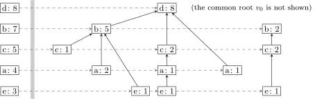
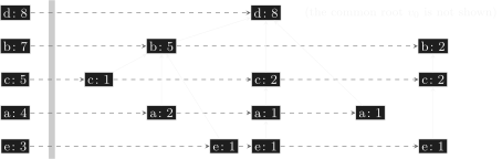
The FP-tree for the example: the levels in decreasing order of support, the total counters of the levels on the left; arrows lead from child vertices to parent vertices, the dashed line links vertices of the same level.
But I claim that this structure by construction contains complete information about all the frequent itemsets. Why? Because all the time we remembered in each vertex's counter how many times we passed through it. Let us check: the sum of the counters on each level always coincides with the counter we filled in in advance for each feature. We really did go through the whole transaction database and lost nothing: the sums agree, that is, we counted each feature in each object exactly once.
Properties of the FP-tree
Definition (The prefix FP-tree). Each vertex of the tree holds a triple :
- a feature ;
- a set of child vertices ;
- a support counter , the number of sample objects whose word begins with the itemset , where is the path from the root of the tree to the vertex .
Notation:
- are all the vertices of the feature (level) ;
- is the sum of the support counters of the feature .
Properties of an FP-tree built from the whole sample :
- is the support of the feature ;
- contains the information about for all frequent itemsets .
Let us introduce notation and at the same time realise what the properties of this FP-tree are and why it really does contain complete information about all the frequent itemsets. Each vertex of the tree we will denote by . Three things are stored in a vertex. The first is a feature: one feature per vertex; moreover, all the vertices of one feature are stored on one level of the tree. Next, an internal vertex has a set of child vertices; note that the tree is not binary at all: there can be any number of child vertices — one, two, three, there are lots of such examples here. And finally, a counter is stored in the vertex.
What is this counter? Can we say that, for example, the counter in the vertex under is connected with some set of features? We can. If we climb from this vertex to the root of the given subtree, we get some subset of features — here — and the counter says how many objects went along this path, that is, how many words begin with . This is not yet the support of the itemset in the whole sample: the itemset also occurs in the word , which went along another path, through the vertex . So to find out the support of an itemset, one has to collect the counters from all the paths where it occurs — we will come to this in a moment. So, the path from the root of the tree to the vertex I denote , and the set of features on this path is . The numbers in the vertices are not simple: each of them is a counter of the objects whose words begin with this path.
Some more notation: are all the vertices of the feature , that is, in fact one level of the tree; is the total support of the feature , the very number we originally wrote on the left: how many times the feature occurs in the sample. And the main property of the FP-tree built from the whole sample: it contains complete information about all the frequent itemsets. Perhaps this is not yet very obvious, although by construction we guaranteed it; let us see why the FP-tree contains information about the frequency of all itemsets and how to get this information out of it.
The support of an arbitrary itemset from the FP-tree
Remark (How to find for an arbitrary itemset from the FP-tree).
- Pick out the paths that contain all the features from , where are the vertices of the lowest level among the features of the itemset .
- Sum the counters of the lower vertices of all such paths: .
Example: — two records, two paths, .
Suppose we have an arbitrary subset of features at the input. How do we compute the support of this ? Very simply. First, we mark all the features that make up our itemset . The levels of the tree correspond exactly to the features, so a subset of features is a subset of levels in our tree. Suppose, for example, we took consisting of the features and . Next, we pick out all the paths each of which contains all the features of this itemset: we look at where in the tree the branches are that contain all the elements of our subset at once. For example, the branch does not contain , so we did not pick it out.
Now we have several branches picked out. What will the support of our subset be? It will be made up of the counters of the lower vertices of all such paths. Why the lower ones exactly? Note: here has a one and has a two. What is this two made of? The first word , where and occurred together. But this two is also made by the word , and there is no there. So to compute the support of , we must take only the paths that contain both and , and take the counters from the lower level, the level of . Such is the rule: in the first step we pick out all the paths containing all the features from , in the second we sum the counters of only the lower vertices of these paths. The claim is that after this we have found the support of the set of features .
The support of the itemset : two paths containing and ; the counters of the lower vertices, , give (slide).
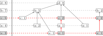
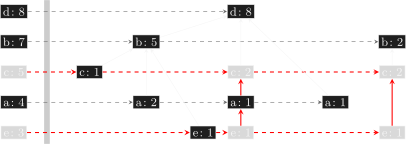
The paths containing the features and are highlighted in red; the support of the itemset is the sum of the counters of their lower vertices on level : .
In this simple way the support of any subset of features can be determined from the tree. Yes, it is a computation, but not a very laborious one, because our tree is not gigantic — precisely because it is a prefix tree, which contains all the information about all the transactions rather compactly.
So we have seen that our structure, the prefix tree or frequent pattern tree, contains complete information about the frequency of all itemsets. We have understood how to build it, but so far by example. Let us turn this into pseudocode and make sure we have understood it well enough to implement it.
The FP-growth algorithm
Definition (The FP-growth algorithm). Input: , the training sample.
Output: the FP-tree ; for all vertices .
Order the features by decreasing .
Stage 1: building the FP-tree from the sample .
- for all :
- ;
- for all such that , in decreasing order of :
- if there is no child vertex , then
- create a new vertex ; ;
- ; ; ;
- ; .
Stage 2: recursive search for frequent itemsets in the FP-tree :
- .
We have two stages: the first is building the FP-tree, the second is finding all the frequent itemsets in the built tree. We will put the second stage aside for now. There will be a function FP-find that works recursively, calling itself, and does roughly what I showed: it must go through all possible subsets of the levels of this tree in some efficient way.
First let us deal with the construction, which we have already gone through by example. We go through all the objects of our sample, passing through each once — a loop over all objects. Next we take the root of the tree. By the way, although I called the vertex and the vertex roots here, there is in fact also a common root, which is not shown. When we have a forest of trees, let us join their vertices by an abstract root that corresponds to no feature, and always start the search from it. This is a purely technical point: is the common root for all these subtrees.
Now we go through all the features that occurred in , and we go through them in decreasing order of support — which is the same as saying that we go down the levels of the tree from top to bottom. If we see a feature , and on the current level of the tree under the current vertex there is no vertex with this feature — remember, when at the very beginning we looked at the word , the first thing we did was create and create — then we create it: we create a vertex in the tree, write our feature into it, and link it with the parent vertex, that is, with the vertex we have just come from. If we are now looking at the first feature, the parent vertex is the common root . The counter of the number of times we have passed through this vertex is zero for now, and it has no child vertices yet. And then, regardless of whether the vertex was old or has just been created, we add one to its counter. These counters can be normalised at once, or the normalisation can be computed later: we start accumulating a counter of how many times a path from the root has passed through the given vertex. That is really all: formally written in pseudocode is exactly what we have just gone through by example, transaction by transaction.
Stage 2: recursive search for frequent itemsets
Remark (Two ideas for an efficient implementation of FP-find). finds from the FP-tree all the frequent itemsets that contain the frequent itemset and adds them to the list .
- Instead of it suffices to pass the conditional FP-tree , the FP-tree generated by the subsample .
- We will add to only the features that are higher in the FP-tree. This way we go through all the subsets .
Let us go on; the most interesting part is ahead: how we will go through all possible sets of features, that is, all possible subsets of the levels of our tree. What will this procedure be? It has three arguments: from the tree it finds all the frequent itemsets that contain a given frequent itemset and adds them to the list . We will now arrange on the set of levels of this tree something like the same breadth-first search. Here we have the itemset , and we have already realised how to compute its support from the tree quickly. Picking out a subset, we can always compute its support quickly. And then we will add to this subset of features, in all possible ways, the features that remain higher in this tree. So we need a recursive function that adds new features to a given in all possible ways — but only from those that are higher than the highest feature of . This will be the way to go through the set of all subsets of the levels of the tree, that is, in essence all possible subsets .
Example : the itemset was chosen from the levels ; we will add to it only the features located higher, and (slide).
Why is it organised exactly so, why do we go through the tree from the bottom up and why in exactly this order? Because there is a very efficient way of finding a certain subtree — we will call it the conditional FP-tree — generated by all the objects on which already equals one. Look at this picture: we have already built , and now we want to check whether some more features lying higher in the tree can be added to . The features that have already entered determine our support: this means that we are now considering the set of transactions in which the features of already occur together. Imagine the whole transaction database, from which you have chosen only the objects where occurs. Clearly such a subset of objects is much, much smaller: each time, by adding one more feature, we greatly reduce the number of objects that contain this feature.
Let us imagine that from this set of objects, which is much smaller than the whole transaction database, we have built an FP-tree — in the same way. It too will be much smaller, very much cut down, and it is in this cut-down, or conditional, FP-tree that we will look for new features to add to . An intermediate structure appears, called the conditional FP-tree: it is the tree that could have been built from the subsample of the objects for which already equals one; this is simply a definition. And we will have a very efficient way of building this conditional tree. Running ahead, I will say that the conditional FP-tree is always a subtree of our main tree: it can be made from it by discarding some vertices, and this discarding is always implemented very efficiently. Moreover, it leads to a conditional FP-tree much smaller than the original, and so the algorithm will work very efficiently.
Definition (The function FP-find). Function .
Input: an FP-tree , a frequent itemset , a list of itemsets . Output: add to all the frequent itemsets that contain .
- for all over the levels from the bottom up:
- if , then
- add the frequent itemset to the list ;
- , the conditional FP-tree;
- find from all the frequent itemsets that include and : .
The conditional FP-tree can be built quickly, using only the FP-tree and without looking into the sample.
Let us implement this idea and look at it in more detail. So, the function FP-find takes as input an FP-tree — to begin with this will be the full FP-tree, and then we will call it passing conditional FP-trees — a frequent itemset , and a list of itemsets . Our task in one iteration is to add one more feature to in all possible ways, and if, adding features, we still get frequent itemsets, to add them to the common list.
What do we do? We go through all the features, over the levels from the bottom up, and check whether the feature has support in the given tree: whether the itemset is frequent. If it is, we add it to the list. We can do this quickly, because we already know how to compute the support of an itemset from the tree: pick out a subset of levels, pick out all the paths where these features occurred, and on the lowest level sum the counters stored in the vertices. In a conditional tree it is even simpler: all its objects already contain , and the support of is simply the sum of the counters of the level .
So, if the itemset is frequent, we add it to the list, and now we build a new tree — the conditional FP-tree conditioned on the given feature. How we build it we will work out a little later: it is very easy to do, but it will need to be looked at in more detail. And now we find from this conditional tree all the frequent itemsets that include both and the feature , that is, we recursively call the function FP-find, where is a tree substantially smaller than the original , and , on the other hand, has grown by one more feature. So the recursion will not be too deep: its depth will never exceed the number of levels in our tree, because each time we add one more feature to .
The conditional FP-tree
Definition (The conditional FP-tree). Let the FP-tree be built from a subsample .
The conditional FP-tree is the FP-tree generated by the subsample , with all the vertices of the feature and below removed.
Now the last non-trivial point of this algorithm: how to build conditional FP-trees quickly. By definition the conditional FP-tree is the tree we would have built if the transaction database contained only the records where equals one. But of course we will not build it anew: we will get the conditional FP-tree from the current tree, and this can be done quickly and cheaply.
Let us show by example how a conditional FP-tree is built from a given one. Here we have an FP-tree, and we want to make from it a conditional tree conditioned on the lowest feature . What must we do? Look at the definition: the conditional FP-tree is the tree built from the transactions involving the feature . The information about all such transactions is stored in this tree on the paths from the vertices to the root. How many such paths are there? As many as there are vertices on the level : occurred three times. So we will get the conditional FP-tree if we take all the paths from the vertices of the lowest feature to the root of the tree and discard everything else.
They must be taken carefully, taking into account what the values of the counters will be. The values of the counters will change: now they must take into account only the transactions in which the feature took part. How will we do this? We will go along all these paths from the bottom up, each time passing the counter from bottom to top. The vertex will now have not a five but a one: will pass a one to this . Why? Because we are interested only in the cases where occurred together with . All the other four were without the feature : there was , there was , there were two — together they made up the five here, and of them we are interested only in the one transaction where too was one. So in the cut-down tree will have a one. In effect we raise the counters from the lower level along the paths from the bottom up, and if paths happen to merge, the counters are summed at that point: thus ones arrive at the vertex from and from , and the result is a two. After that the lower level can be removed, because we have already taken the feature into account: in a conditional FP-tree, the level of the feature it is built on is no longer there.
The conditional FP-tree (blue) is obtained from the paths from the vertices to the root (red); the counters are raised from the bottom up, and the level is removed (slide).
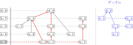
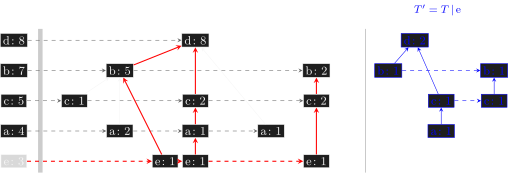
On the left, the FP-tree with the paths from the vertices to the root highlighted in red; on the right, the conditional FP-tree : the counters are raised from the vertices from the bottom up, and the level is removed.
Let us check: does this FP-tree really contain the information about the three transactions involving the feature ? There were three, and they are indeed all accounted for: the counter of is two, that of is one; together they add up to three. This tree really does record complete information about all the transactions involving the feature .
Definition (Fast construction of the conditional FP-tree). Input: an FP-tree , a feature . Output: the conditional FP-tree .
- Keep in the tree only the vertices on the paths from the vertices of the feature upward to the root : .
- Raise the values of the counters from the vertices from the bottom up by the rule for all .
- Remove all the vertices of the feature from .
Only the features above remain in the tree , because at the moment FP-find is called all the itemsets containing features below have already been looked at.
We have in fact come almost to the end of this really not very simple algorithm. Let us do the last thing: write in pseudocode the algorithm for building a conditional tree that we have just gone through by example. In essence there will be no loops here, three simple steps. At the input are the tree and the feature , and we want to build the conditional tree . The first step: we keep in the tree only the vertices on the paths from the vertices of the feature upward to the root. This is what we did for : we found all its vertices and laid paths from these vertices to the root — thereby building the skeleton of the conditional tree. Second: we raise the values of the counters from the vertices corresponding to the feature from the bottom up and use the summation rule: if two paths meet at a vertex, we sum the values of the counters there. And the third step: all the vertices of the feature itself are removed from the conditional tree, because we have already taken them into account earlier; their supports are already counted.
Why so? We can go back to the picture with the levels. We always consider some subset of features and try to add to it new features that are located higher in the tree. This means that when we consider the conditional tree conditioned on the subset , we have already taken into account all the frequent itemsets that contain these features, and we are now trying to add a new feature to all these frequent itemsets. This is simply a mechanism for going through all the subsets of the levels of this tree, and we always go through them from the bottom up.
That is the whole algorithm. Let us run through it once more in retrospect. The first thing we did was build the FP-tree in one linear pass over the transaction database. Second, we start FP-find with the full tree, the empty set and the empty set: we start growing frequent itemsets from scratch and start filling the list of frequent itemsets . Then we go through the features from the bottom up: as soon as we have removed the lowest feature, we start adding one of the upper ones to it. In this way we gradually go through all the subsets of the levels of this tree, and that is the same as all the subsets of the set of features.
The efficiency of FP-growth
The of the algorithm's running time as a function of MinSupp, compared with other algorithms (on the census data); the lower curves are two different implementations of FP-growth. Christian Borgelt. An Implementation of the FPgrowth Algorithm. 2005.
And the final plot, from a paper on the implementation of this algorithm: it shows how much faster this way of finding frequent itemsets is than simple algorithms. Here the upper curve is APriori, the lower curves are two slightly different implementations of FP-growth. On the horizontal axis is MinSupp, on the vertical the logarithm of the time needed to find all the frequent itemsets. First, clearly, as the support grows, the number of itemsets decreases and the time decreases. But note that on the logarithmic scale the time of FP-growth comes out much smaller than that of the other algorithms.
Remark (A question: is the conditional tree built for one feature or for a subset?). — Do I understand correctly: first we build the FP-tree, then we pick out a subset, for example with , find the frequency of occurrence of this subset, and then strike it out of the tree in order to study the other subsets that lie higher?
On the whole, yes. Look: in the picture with the levels the set is a set of several features, and they need not be consecutive. The tree in my example is small, only five levels, but in general is a subset of some features, and at each iteration you try to add to this subset one more of the features located higher. This way you will go through all the subsets. When you build a conditional tree, you always cut the tree down by one feature: you take some feature, throw it out too, get the next reduction of the tree, and continue trying to add features using this reduced tree.
Clearly it is not necessarily the last feature that can be removed. When you go through all the features, is the current conditional FP-tree; only at the first call, at the first iteration, is it the whole tree you had originally, and at all the other entries into this function you are considering some conditional FP-tree and moving through all the levels of this tree. The picture with the conditional tree is drawn for excluding the lowest feature , but in the same way you will try in turn to exclude , and , and . And each time there will remain, first, only the features above the excluded one, and second, only the features you meet on the paths from the vertices of the excluded feature to the root of the tree.
— And if we take, say, the subset , can we do it at once?
No, look: in this picture you exclude only one feature. You now have a subset , and you form a subset that will have one feature more. For this you must try adding , then , then , then . Each time you will in effect have this task: from the tree you have now, you exclude and get a new conditional tree, the blue one; then you exclude and get another blue conditional tree, in which there will be neither the level nor the level ; then you exclude , and so on. Each of these features is excluded in turn, and this guarantees that you will in the end go through all the subsets of features.
In principle one could work without conditional trees: a simpler algorithm is possible, which just as well goes through all the subsets of features from the bottom up and computes all the supports from the tree. This is easy to do, but then you will have to work with the full tree all the time. Introducing cut-down conditional FP-trees makes the algorithm much more efficient, because at each next iteration you work with a tree that is substantially smaller than the previous one, yet is a part of it.
Summary
Remark (Summary).
- Association rule mining is unsupervised learning.
- An association rule is (by definition) almost the same as a logical regularity.
- Simple algorithms like APriori are computationally inefficient on big data.
- FP-growth is one of the most efficient association rule mining algorithms.
- Practical applications use its incremental and/or hierarchical generalisations.
We have come to the end. A brief summary. Association rule mining is, first, a kind of logical classification algorithm based on conjunctions, only here we have classification without a teacher: which class to classify against is also built into the problem; the role of the class is played by the subsets , which we also construct. The FP-growth algorithm was invented quite long ago, but in effect it still remains the state of the art and one of the fastest association rule mining algorithms. And for practical applications a great many of its generalisations have been devised — for hierarchies, for increment and decrement, and so on.
No comments yet
Be the first to share your thoughts.