August 30, 2026 · Lecture · LibreTimes
Machine Learning 2. Lecture 7. Recommender Systems
Contents
- What this lecture is about
- The formulation of the problem and applications
- Definitions and notation
- Examples of applications
- The Netflix Prize competition
- The main approaches in collaborative filtering
- Correlation models
- User-based and item-based collaborative filtering
- Similarity functions
- The sparse linear model SLIM
- A summary of memory-based methods
- Latent models and matrix factorisations
- Low-rank matrix factorisations
- The singular value decomposition (SVD)
- The alternating least squares method (ALS)
- The latent factor model (LFM)
- Nonnegative matrix factorisations (NNMF)
- Probabilistic latent semantic analysis (PLSA)
- Taking implicit information into account (implicit feedback)
- Taking additional information into account
- Autoencoders for collaborative filtering
- Matrix factorisation as a linear autoencoder
- Neural network autoencoders
- Additional data in matrix factorisations and autoencoders
- Factorisation machines
- Hypergraph models
- Evaluating the quality of recommendations
- The precision and recall of recommendations
- Diversity, novelty, coverage and others
- Offline and online quality
- Summary
- Seminar
What this lecture is about
Today we consider recommender systems, collaborative filtering and matrix factorisations. The plan is fairly packed: this is a well-developed field with many different methods. We will begin with simple ones, continue with advanced ones and finish with quality metrics, about which we will manage to say only a little.
The formulation of the problem and applications
Definitions and notation
There are two finite sets. They are called differently; in the English-language literature users and items have taken root. Sometimes users are called subjects and items objects, sometimes users are called clients; the terminology wanders, but the English one is more settled. For brevity I will say "clients" and "items".
Definition (Definitions and notation). is the set of clients (subjects, users); is the set of items (goods, objects).
Types of input data:
- , transaction data, the space of descriptions of transactions;
- , the matrix of relations (or cross-tabulation), :
- , binary data;
- , ratings (ordinal or integer).
Problems in recommender systems:
- filling in missing values in the cells ;
- ranking a list of top- recommendations for or for .
Something happens between these two sets: for example, clients buy, choose, like some items, and our problem is about these interactions. Formally the input data are transactions: a client bought some product, liked it, did something. The user's actions in some systems may also be varied. It is one thing to go to a car dealer's site and gawk at cool cars; another to look at a particular make of car on different sites, and then it already seems that you are going to buy it; a third when the user has gone to the dealer's site, to the contacts, and looked up the telephone number or address: evidently he is already about to come and make a purchase. That is, transaction data are knowingly more varied than what we usually work with later.
Usually we work with the matrix of relations between these two finite sets; it is also called the cross-tabulation matrix, or the user–item matrix. is the result of aggregation: we take a particular client and a particular item , everything that happened between them, views, purchases, likes and so on, and aggregate it into some quantity. There are different situations: it may simply be a binary quantity, bought or did not buy, viewed or did not view, if it is about page views; and if it is about books, films, that is, where the individual tastes and preferences of clients are expressed, may be a score, a rating the client gave the item.
We can guess several properties of this matrix at once. First, it is sparse, and strongly so: there may be millions of clients, millions of items, and it is unlikely that every client has done something with every item. We will have to consider several cases: sometimes the data are binary, sometimes real-valued, sometimes ratings, and ratings are ordinal data: we understand that a rating scale is subjective, and most likely a three differs from a two not in the way a five differs from a four; in some models this too is taken into account explicitly. The main problems here are either predicting the unfilled cells of the matrix, that is, whether the item will interest the client , or forming a ranked list of personal recommendations of items for the given client; this already resembles the ranking problem we studied last time.
Examples of applications
Example (Recommender systems for e-commerce). are the clients of an online shop; are the goods (books, video, music, courses, events, etc.); .
Problems of personalising offers:
- filling in missing values in the cells ;
- ranking a list of top- recommendations for the client ;
- finding a collaboration (collaborative filtering);
- targeting offers (cross-selling, up-selling).
For example, the clients of an online shop buy some goods: books, video, music and so on. Recommender systems are needed most often where different people have different tastes, and one has to recommend to a client what he will like with high probability and what he will choose; in this way one can increase the turnover and profit of the online shop. The problems of personalising offers are not reduced only to predicting unfilled cells or ranking recommendations. For business such problems as cross-selling and up-selling are also of interest. Cross-selling: the client is already about to buy something, and we can offer him something else, and perhaps he will not refuse. At that moment the question arises: what to offer him so that he buys this too with high probability, that is, increases our sales? Up-selling: how is the client to know about a new product that has appeared with us? Offers of new goods somehow have to be built into the recommendations.
Examples of recommender systems by category: video, news, music, social networks, e-commerce (slide). Rui Chen et al. A survey of collaborative filtering-based recommender systems: from traditional methods to hybrid methods based on social networks. 2018.
There is a huge number of applications; I took this little table from the paper I refer to simply to show how many different recommender systems are used all over the world: for recommending video, music, news streams, in social media and in e-commerce, in online shops.
Example (A recommender system for web pages). are internet users; are text documents (sites, pages, news, etc.); is the vocabulary of words (tokens, terms) making up the documents; ; is the frequency of the word in the document .
- Web Content Mining: analysing data about content ();
- Web Usage Mining: analysing data about usage ().
The main hypothesis of WUM: the user's actions characterise his interests, abilities, habits, tastes.
Problems of personalisation: find relevant documents for a user, a document or a selection of documents.
The second example is a slightly specialised class of problems, when we recommend some text documents to internet users: sites, pages, news and so on. Texts are items of a certain kind that consist of words, and this too can be used. The interaction between the two sets of users and items is joined by a third, the set of words of which the documents consist, and interactions between documents and words appear. Our sparse matrix can be regarded as a bipartite graph between vertices of two types, clients and items, and here there is one more type of vertex: the words in documents. When we do information retrieval, personalisation of search or of recommendations, we have two possibilities. One can use data about the content: recommend to the user, for example, pages similar to those he has already visited with pleasure. Or one can use data about users and look for collaborations, that is, users similar to ours, who have common preferences, tastes, and are inclined to choose the same items. This is called web usage mining as opposed to web content mining; there are also hybrid schemes, where both kinds of information are used. The main hypothesis in web usage mining is that the user's actions characterise his interests, but not only interests: also abilities, habits and tastes. Our task is to identify similar users and use the information about what they bought to form offers for the given particular user.
The Netflix Prize competition
Example (A rating-based recommender system: the Netflix competition). are the clients; the films; is the rating that the client gave the film .
- 2 October 2006 to 21 September 2009; the main prize, dollars;
- clients, films;
- ratings of films on the scale ;
- the accuracy of the predictions was evaluated on a test sample :
- the task: reduce RMSE from 0.9514 to 0.8563 (by 10 %).
Y. Koren. The BellKor solution to the Netflix Grand Prize. 2009. A. Töscher, M. Jahrer. The BigChaos solution to the Netflix Grand Prize. 2009.
One more very well-known example is in effect the data analysis competition with which the whole movement of competitions began; before it they were entirely one-off and rather rare events. In 2006 the company Netflix announced a competition to improve the quality of rating prediction. At that time 70 per cent of the company's revenue came from purchases made through recommendations, and for their business it was very important to improve the quality of recommendations. Everything in this competition was interesting. First, the prize, a million dollars; this was unprecedented, nobody had offered such prizes for solving data analysis problems until then. Second, the competition lasted almost three years, and although the conditions required improving the quality of predictions by only 10 per cent, in these three years the scientific community understood practically everything about collaborative filtering problems and matrix factorisations for recommendations; it really was a breakthrough in science. When the organisers, after the end of the competition, gave presentations about how it had all gone, they honestly admitted that for such a ridiculously small sum they would never in their lives have got such a huge community of postdocs all over the world to work for them: the prize was ridiculously small compared with how many interesting insights they got.
The data are large, but not super-large: about 480 thousand clients and about 18 thousand films, ratings on a five-point scale from 1 to 5, and the ratings had to be predicted on a test sample, also fairly large. The metric was in fact not a very fortunate one: ratings are, it seems, an ordinal scale, and they decided to use the root-mean-square metric, and that was the most unfortunate decision in this competition. For recommendations it is of course interesting to evaluate the quality of the list of recommended films; that would have been much closer to their business. But the community in effect got hooked on this metric and used super-complex methods to squeeze out some tenths and hundredths of a per cent; from a substantive point of view this was not entirely adequate. Today we will often recall these data and the methods developed in the course of the competition, and refer to the winners, the teams that took first and second place.
The main approaches in collaborative filtering
Remark (The main approaches in collaborative filtering (CF)). By the mathematical technology used:
- correlation models (Memory-Based CF): correlations of the rows and columns of the original matrix ;
- latent semantic models (Latent Model-Based CF): vector representations (embeddings) of clients and items.
By the types of data used:
- 2D: only the matrix (in particular, the Netflix competition);
- 3D: context-dependent (context-aware, field-aware);
- taking the content into account (content-aware, hybrid models);
- taking trust links between clients into account (trust-aware);
- taking time into account (time-aware).
F. Ricci, L. Rokach, B. Shapira. Recommender Systems Handbook. Springer, 2015.
It is already clear where the name comes from: we build a collaboration, that is, a set of people whose preferences and tastes are similar to those of the user for whom we are now making a recommendation. There are two main techniques. The old ones, considered outdated, are correlation models, memory-based, based on storing the whole original clients–items matrix in full and looking for correlations between rows and columns. And the more modern ones are latent models, which build compressed vector representations for clients and items. We already understand that this may be topic modelling or the singular value decomposition, we will do a lot of matrix factorisations today, and in terms of neural networks these are autoencoders; we will recall them today too.
One more important point: by the types of data used, the methods also divide into a fairly diverse set. The basis is considered to be the so-called 2D models, two-dimensional because they are based on analysing the clients–items matrix, and there is no other information. When some information about the items or the clients appears, feature descriptions, some context, information from the subject area, these are already called 3D models. Further, there may be hybrid models, models that take into account interactions between clients, if it is a social network, they may also communicate with each other, and models that take dynamics, time, into account. All these are various additional data that can be used to improve the models and remove their drawbacks; we will manage to talk about this a little at the end.
Correlation models
User-based and item-based collaborative filtering
Let us begin with the simplest: correlation models, based on storing the matrix in full. There are two approaches here: either we work with the rows, the rows are clients, and this is called user-based collaborative filtering, or with the columns, the items, and this is called item-based. Since we have a matrix, there are two views of it, by rows or by columns, and correspondingly two approaches, client-oriented and item-oriented.
Definition (Nonparametric regression for filling in missing values). Estimating a rating from similar clients (User-Based CF):
is a collaboration, the set of clients similar to ; is the mean rating of the client ; is the similarity function of a pair of clients .
Estimating a rating from similar items (Item-Based CF):
is the set of items similar to ; is the mean rating of the item ; is the similarity function of a pair of items .
We want to predict a missing value, that is, an empty cell: we do not know how the client relates to the item , and we want to predict it. The prediction is in effect the Nadaraya–Watson formula, which you know from last semester. One subtle point: we predict not the rating itself, not the score itself, but its deviation from the mean. What for? Different clients have different subjective attitudes to a point scale, first of all a scale of the type in the Netflix competition, 1, 2, 3, 4, 5. Some give all films four or five, some two or five; people perceive the scale of school marks very differently; some never give a one, just as for some reason ones were not given at school, while for a rating that too is a perfectly good score. To fight the clients' habits, we introduce a mean rating for the client and predict the deviation from the mean. Otherwise it is simply the Nadaraya–Watson formula: we try to predict the row of the matrix corresponding to the client from all the other rows. Remember ordinary regression? Only here the matrix has to be transposed: in ordinary regression the rows were objects and the columns features, while here other clients, their rating vectors, act as features. And somehow the similarity of a pair of clients, that is, of a pair of rows of the matrix, has to be estimated. The item-based approach is exactly the same up to transposition: columns are predicted, that is, in terms of "objects–features" the users act as objects and the goods as features; the formula is exactly the same in appearance.
Similarity functions
Definition (Similarity functions for rating data). is the set of items the client has rated; is the set of items rated by both and .
Pearson correlation:
The cosine similarity measure:
where it is implicitly assumed that if .
The similarity function of pairs of items is defined similarly.
How is similarity sought in the case of rating data? We quite often subtract the mean, and in this case we define the Pearson correlation between rows, between clients, subtracting the mean for each client; the Pearson correlation is a very natural measure here, which takes precisely these corrections for the mean into account; it is simply the ordinary classical correlation. Sometimes the cosine similarity measure is computed, that is, the cosine of the angle between the two vectors defined by two rows of the matrix.
The question arises, of course: we agreed that the matrix in most real applications is strongly sparse; how, then, are correlations to be computed? Note: the sums are computed over the sets of items that both users have rated. We have, as it were, laid two rows on top of each other like filters and singled out only the set of items that both have rated. It may well turn out that this intersection is empty altogether. Nothing terrible happens: if we are making a prediction for the user , and the user differs from him so much that they did not coincide in ratings on a single item, then certainly need not be taken into account: he is not in the collaboration for . On the contrary, we have, so to speak, made use of the sparsity of the matrix to reduce the computations.
But summation over the sets of rated items implicitly comes down to the assumption that a missing rating equals zero: if a client has never seen an item, the rating for him is, as it were, 0, and this seems to be interpreted as the item being of no interest to the client, which of course is not so. An implicit assumption is made that the items the client has seen interest him, and all the others most likely do not. Most likely that is so, but among them there should still be those for which we will predict high ratings. There is a certain drawback of these similarity measures in this, and very many methods are aimed at working with the sparsity, at taking these implicit zeros into account. Whether they should be taken into account or not depends on the problem; we will touch on these details several more times.
Definition (Similarity functions for binary data). The larger , the more similar the clients and .
The Jaccard similarity measure:
Fisher's exact test (Fisher's Exact Test, FET). The probability of the overlap of choices under the null hypothesis that the clients and make their choice independently, , :
The sets of items chosen by the clients and , and their intersection (slide).
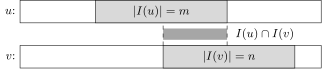
The rows of the binary matrix for the clients and (the items are ordered conventionally): the chosen items are shaded, and their intersection is the dark strip between them.
And what to do if the data are binary? How is proximity to be measured in this case? There are many proximity measures; the simplest is the Jaccard measure. If we have a client with his set of ones in a row of the matrix and a client with his, there is their intersection, and of course one has to measure how large this intersection is compared with their union. This is a natural, intuitively clear measure: if two clients have similar interests, the intersection will make up a large share compared with the union of these two sets.
But one would like to estimate this in a more grounded, statistically literate way, and here Fisher's exact test comes to the rescue. It tests the null hypothesis that the ones of the client and the ones of the client are two independent random binary quantities. If the ones here and there are generated independently of each other, it is clear how to estimate what the cardinality of the intersection will be: it is the hypergeometric distribution, and the probability that there will be exactly ones in the intersection is written by it. The larger the intersection, the smaller the probability that it could have formed purely by chance under the null hypothesis of the independence of and . That is, and are in one collaboration, useful to each other for prediction, if there are anomalously many common ones compared with the number there would be under the null hypothesis that and make their choice independently, that they have no common interests. So minus the logarithm of this probability may serve as an adequate criterion of the informativeness of the intersection: if it is too large, it means we have information that the interests of and are after all dependent.
The story about simple correlation models ends here. Everything is very simple: we take the matrix, measure the correlations between rows or between columns, use the Nadaraya–Watson formula, and that is all. The drawbacks of these methods are clear: it is unclear how to choose the correlation measure, it is some heuristic, and one has to process this matrix in full all the time.
The sparse linear model SLIM
In the end these methods were abandoned in favour of latent matrix factorisations, but there is one very interesting method that lies somewhere on the border. It is still a memory-based method: it is based on storing the matrix in full, and no latent vector representations are built here. Nevertheless it turned out to be very successful and is even considered one of the state of the art in recommender systems. This is the so-called sparse linear model, SLIM.
Definition (The sparse linear model (Sparse Linear Method, SLIM)). Given: , a (strongly) sparse matrix.
Find: linear regression models (item-based) instead of a nonparametric regression with an untrainable function :
Criterion: the method of least squares with and regularisers, with a non-negativity constraint on the coefficients and the condition that an item must not be estimated from itself:
Xia Ning, G. Karypis. SLIM: sparse linear methods for top-N recommender systems. 2011.
Recall the formula of the item-based approach: we estimate the column of the matrix corresponding to the item ; we go over all the other items , find the close ones among them and average the ratings of these close items. This is very much like a linear regression model, and so the idea arises: let us explicitly predict some columns from others, predict the column of the matrix from all the other columns by linear regression. In this linear regression the coefficients are , that is, is a square matrix; in the user-based approach its size would be . It is interesting that for each item, for each column, we build an independent linear regression; this is well seen in the matrix notation: the estimate for a column is simply the original matrix multiplied on the right by the vector of parameters of the linear model. It would seem a very simple, natural approach that rather obviously suggests itself, especially after we have understood that the item-based approach in correlation models is nothing other than the Nadaraya–Watson nonparametric regression. So let us use parametric linear regression: a very natural model.
Of course we will use the method of least squares, and at once take regularisation so that there is no multicollinearity; we already know that there is the neat elastic net method, in which two regularisers are used; let us use it. We will also impose constraints. The coefficient in effect speaks of the similarity between and , and it is natural to assume that this analogue of a similarity function should be non-negative. And there should be zeros on the diagonal of the matrix : we have no right to estimate an item from itself; an item must be estimated from all the others. This is an important constraint. We get a not quite standard regression problem, with a small peculiarity in the form of these constraints.
Remark (The advantages of SLIM).
- It is a standard linear regression problem (ElasticNet).
- The solution parallelises over the columns , .
- regularisation makes the solution sparse.
- Additional feature selection by the cosine measure: for each we take the 10 features with the largest .
- A successful method in ranking quality and speed.
So, it is elastic net. The second thing that is very good is that the method parallelises completely over the columns: regression problems independent of each other are solved. The regulariser promotes sparsity, that is, we will get a model that itself says which items are important for predicting the ratings of the given item: for each item we explicitly build a model of its similarity. It is good that we do not have to invent the similarity function : it is the result of the linear model, its coefficients, which is remarkable in its own way. And it is also interesting that additional sparsing can be introduced: besides regularisation, explicitly select the most suitable features for predicting each item , that is, form the set of features with the largest proximities. It is proposed after all to compute the proximities and use them for such a rather crude feature selection, and it turned out that it is enough to take 10 features, while attempts to increase them to 100 or 1000 lead to nothing special: it is enough to take a relatively small number of features for each product.
The dependence of the LOOCV HitRate on the length of the recommendation list on the Netflix data for SLIM and other methods (slide). Xia Ning, G. Karypis, 2011.
The method turned out to be quite successful. Here are graphs from the paper where SLIM was compared with various other models, both correlation-based and based on latent representations, and nevertheless this method turned out to be competitive and beats many other methods.
A summary of memory-based methods
Remark (A summary of memory-based methods). Advantages for business applications:
- easy to understand and explain: "those who bought this book also bought…";
- easy to implement;
- the SLIM method is simple and still one of the best.
Drawbacks:
- the huge sparse matrix has to be stored;
- the "cold start" problem: it is unclear what to recommend to new clients; unclear how and to whom to recommend new items;
- sometimes the recommendations are trivial: everything most popular is offered.
Next: how latent models remove these drawbacks.
To sum up: all this was the story about memory-based methods; the matrix is stored in full, in its original form. The advantage is that the methods are not complicated; even SLIM is fairly simple, because it uses standard ready-made approaches, linear regression. And it is easy to explain to the client how the recommendation comes about. One of the first large online shops started by forming recommendations even without any of these methods, literally implementing a simple rule: "users who bought this book also bought…", followed by a list of recommendations. They literally looked for users who had bought the same book; this is done by two SQL queries. Later the methods were improved, first correlation methods were used, then latent models, but the wording was kept: it was clear to users, and when we make an offer, the user understands what is being offered to him.
The drawbacks of memory-based models: first, the matrix has to be stored in full; second, there is the so-called cold start problem. If a client comes to us for the first time, he has not yet made any choices, and it is unclear what to offer him. If an item is a new product that has not previously been sold on our platform, it is unclear to whom to offer it, because we have no information about who has bought it. To overcome this problem one needs, of course, additional information, about the clients, about the items or about both, so as to understand something from indirect data about the clients' preferences and about which interests of clients the items are able to satisfy. And many such approaches give rise to trivial recommendations: if we talk about books, everyone is recommended "Harry Potter", because it is the most popular book. Now we will remove these drawbacks.
Latent models and matrix factorisations
Low-rank matrix factorisations
We move on to the main thing I would like to tell about in today's lecture. To be honest, for me recommender systems are only an occasion to tell about matrix factorisations: what kinds there are, how different they are. Of course, they are applied not only in recommender systems; their application is much wider, in completely different applied fields: biology, geology, sociology, wherever you like. But we will go on reasoning in terms of clients and items, although it is clear that we are dealing with a huge matrix for which a representation has to be built that is able to predict the missing cells: matrix completion.
Definition (Low-rank matrix factorisations (matrix factorization)). Given: , a (strongly) sparse matrix.
Find: , the set of interests (topics), ;
- , the row is the vector of interests of the client ;
- , the row is the vector of interests of the item ;
Criterion: .
Methods of solution:
- the singular value decomposition (SVD);
- nonnegative matrix factorisation (NNMF): ;
- stochastic matrix factorisation (topic modeling).
Latent models are based on the idea that each client and each item can be assigned a vector of interests. Interests are the same as topics in topic modelling, but here they are more often called interests. Each client is characterised by a vector of interests, what interests him, and each item by the same kind of vector, which interests of people the given item is able to satisfy. Collecting all these vectors, we get two matrices: the matrix with elements , whose row is the vector of interests of a client, and the matrix , whose rows are the vectors of interests satisfied by the given item. Our task is to find a matrix factorisation. Why precisely a matrix factorisation, why the scalar product of the -th row of the matrix with the -th row of the matrix ? Very simply: why will the client choose the item ? Because his interests coincide with it, because the item is able to satisfy the very interests the client has; a high correlation between these vectors means that the item suits the client, they have a common interest. In matrix notation we build the matrix and want it to approximate the original . The norm here can be understood in different senses; in particular, if the matrix is sparse, we will form the norm not over all the cells of the matrix but only over those where the values are known.
There is also a probabilistic interpretation, which in effect says that topic modelling can be used to solve this problem. Its substantive interpretation is very clear: the client is characterised by his profile of interests, a discrete distribution on the set of interests. One can even say this: a user has come into our online shop, and the probability that he is interested in some topic is described by this distribution. And for each interest there is a distribution over all the goods of our online shop, the probability that the interest can be satisfied by the product . And the total probability formula estimates the probability that the client will buy the product from us. A very natural model, but it imposes additional constraints on the matrices and : the interest profiles, the rows of the matrix , must be normalised, and the columns of the matrix must be normalised as discrete probability distributions, normalised and non-negative.
To solve the matrix factorisation problem one can use classical methods of the singular value decomposition type, we will begin with that; one can use nonnegative matrix factorisations, where there are non-negativity constraints; additionally one can impose normalisation constraints, and then a probabilistic meaning arises in the whole model: our interest profiles become interpretable, we understand which items each interest consists of and can interpret it. These are already topic models. Three main types that can potentially be used to solve this problem; let us go through them in order.
The singular value decomposition (SVD)
Definition (The singular value decomposition (SVD)). The least-squares criterion: .
The singular value decomposition:
Merits: ready-made linear algebra libraries can be applied; good ranking of offers on some data.
Drawbacks:
- if is not known, we set (we implicitly consider that if the client has not chosen the item in any way, it most likely does not interest him);
- the orthogonality of the (eigen)vectors , ;
- the components of the vectors , are not interpretable.
P. Cremonesi, Y. Koren, R. Turrin. Performance of recommender algorithms on top-N recommendation tasks. RecSys 2010.
The first is the singular value decomposition; the classical formulation of the problem from last semester, recall the principal component method. Our matrix factorisation can simply be formed from the singular value decomposition: there a product of three matrices arises, the orthonormal matrices and , and in the middle a diagonal matrix with the eigenvalues on its diagonal. It can be split: the root of goes to the left, the root of goes to the right, and we have a factorisation into two matrices, also orthogonal but no longer orthonormal; only the normalisation changes. The plus is that we have reduced the problem to an already known one for which there are numerical methods, and by and large the singular value decomposition is a fairly successful method that solves some problems quite well.
But there are several drawbacks. First, the matrix usually has missing values, moreover, in the Netflix competition data there were about 99 per cent missing values, these matrices are usually sparse, while the singular value decomposition requires full knowledge of the matrix . Where did the missing values go? In fact they were implicitly replaced by zeros. This is an implicit assumption: if we know nothing about how the client relates to the item , it is a missing value; perhaps he likes it and it should even be recommended; but in building the singular value decomposition we implicitly say that he likes it very little: since he did not choose it, he does not like it. This is wrong, does not correspond to the truth, although in most cases it may well be so. This implicit assumption that missing values equal zero is a bit of a strain, and one would like methods that bypass missing values altogether and in no way try to use them as zeros. Moreover, the orthogonality of the eigenvectors in the matrices and is, as a rule, not interpretable: why they come out orthogonal is not very clear; it is not needed and does not even correspond to the meaning of the problem. And finally, the components are not interpretable: we understand that this is some vector representation, but the coordinates in these vectors have no meaning. Meaning will begin to appear if we do nonnegative or nonnegative normalised matrix factorisations; in topic models these vectors will be interpretable.
The alternating least squares method (ALS)
The next method is also used under the implicit assumption that the empty cells of the matrix equal zero: the alternating least squares method. Also very often used, simple, but far from the best.
Definition (The alternating least squares method (ALS)). The least-squares criterion with regularisation:
The alternation method ALS (Alternating Least Squares):
The problem splits into independent linear regressions (the computations are easily parallelised):
The same optimisation problem as in SVD is solved, but now orthogonality is not required: we simply use a method that minimises this functional, and there will no longer be any orthogonality of the matrices and . Moreover, we include regularisers here at once, so that there is no multicollinearity and overfitting. We differentiate and set to zero the derivatives with respect to and . Having differentiated with respect to and set the derivative to zero, we get for a known , the solution of a least-squares problem; this formula is in effect ridge regression, again we recall last semester, ridge regression for all the rows of the matrix . We do the same for and get for a fixed , also as the solution of a regularised least-squares problem, also ridge regression. The idea is to alternate these computations: for a known compute , and for a known compute . These computations can be parallelised, because they are independent over rows: one can compute the -th row of the matrix knowing the whole matrix and only the -th row of the matrix , and similarly with the columns. The method is fairly simple and fast, there is a heap of ready-made numerical algorithms for it, and so it is fairly popular. Note, by the way: in Russian "alternating" is often illiterately translated as "alternative least squares"; they are by no means alternative but alternating, that is the sense of this English word: we compute for a known and for a known in turn.
But here too there is no bypassing of missing values: linear algebra does not tolerate empty cells in vectors, and if there is a missing value in the matrix , we simply put a zero value there, which is not entirely adequate.
The latent factor model (LFM)
This can be fixed by the following model, called the latent factor model; it is sometimes called sparse SVD, because it is the same functional, essentially the same norm, but the summation is not over all the cells of the matrix but only over those that contain values.
Definition (The latent factor model (LFM, Latent Factor Model)). The least-squares criterion for sparse data:
The stochastic gradient method: we go over all many times in random order and each time take a gradient step for the problem :
One can also train () and () as parameters.
G. Takács, I. Pilászy, B. Németh, D. Tikk. Scalable collaborative filtering approaches for large recommender systems. JMLR, 2009, No. 10, pp. 623–656.
It would seem that nothing prevented us from writing out such a problem before: why fill the matrix with zeros, and increase the computational complexity besides, if there are 99 per cent of these zeros there? So let us go only over the non-zero values and approximate them by the product of two vectors. In effect what is written here is the scalar product of the -th row of the matrix with the -th row of the matrix ; this is what we talked about: two vectors of interests, for the client and for the item, are multiplied, and this is used as a predictive model for . As we said before, subtracting the mean ratings is a certain reasonable normalisation; it can be added or not. The means and can be computed as means, or they can be regarded as trainable parameters of the model and optimised over; there are options.
Clearly, the stochastic gradient method is very natural for solving this problem. We go over at random the pairs corresponding to the filled cells of the matrix and take a gradient step on one term of this sum. It is easy to differentiate, the gradient looks very simple, and we get a very simple iterative process.
Remark (The advantages of the stochastic gradient method for LFM).
- Regularisation is easily introduced: .
- Non-negativity constraints , are easily introduced (the gradient projection method).
- A generalisation to rank data is easily introduced:
where is a smooth monotone function with parameters that transforms the estimates into the rating scale .
- All kinds of incrementality are easily implemented: adding one more client , item , value .
- High numerical efficiency on big data.
It is very easy to build in regularisation, very easy to introduce non-negativity constraints; the gradient projection method is used: as soon as we go into the negative region, we zero the corresponding element. One more modification can be made for rating data. Remember, I said that ratings are subjective: although they are expressed in numbers, usually 1, 2, 3, 4, 5, one cannot say that they can be subtracted from each other, that is, ; there is an order relation, but arithmetic operations with an ordinal scale are in principle inadmissible, and yet we allow ourselves them. How to transform the scale? For example, like this: we still keep the numerical ratings 1, 2, 3, 4, 5, but understand that the model has to be transformed somehow, and we do this with a smooth monotone function with a small number of parameters; usually the number of parameters equals the number of ratings on the scale, from 1 to , that is, parameters. It is a certain monotone spline, a piecewise-constant, piecewise-linear, piecewise-quadratic or piecewise-cubic simple function with a small number of parameters, which in effect brings the values produced by the predictive model to the ordinal rating scale 1, 2, 3, 4, 5. This transformation has to be tuned separately.
The stochastic gradient method also has one useful property: it adapts very easily to the case where the problem is dynamic and new clients and new items may appear. As soon as something new has appeared, it is computed by the same formula; this can be done at some intervals, there are various implementation options, but on the whole, when new elements of the matrix appear, the whole model need not be recomputed from scratch: it can be completed using only the new elements. It is a good, numerically efficient method. I refer to the paper of one of the teams that led the Netflix competition for quite a long time, a team from Hungary; they used this method actively.
Nonnegative matrix factorisations (NNMF)
Let us go further. We are proceeding little by little along the scheme of gradually moving away from the ordinary singular value decomposition, taking additional constraints into account. We have just taken into account that the empty cells of the matrix should not be replaced by zeros but missing values should be bypassed. Now let us talk about how to take into account an additional constraint: the vectors of interests should be non-negative. Then we will get an interpretable model: we will understand exactly that a coordinate of the vector is the degree to which an interest is expressed in the given user or the given item.
Definition (The NNMF problem (Non-Negative Matrix Factorization)). The least-squares criterion for nonnegative matrix factorisation:
Again the alternating least squares method (ALS), but now the columns and then the columns are found in turn, with the rest fixed: :
(the positive cut-off comes from the Karush–Kuhn–Tucker conditions).
A. Cichocki, R. Zdunek, S. Amari. Hierarchical ALS algorithms for nonnegative matrix and 3D tensor factorization. 2007.
How can we include the additional non-negativity constraint in the method of least squares? Let us try to use the same idea as in the alternating least squares method, but a little differently. Before, we computed and , the rows of the matrices and corresponding to clients and items. Here we will compute in turn the columns of these matrices: is the column corresponding to the interest , it consists of clients, and is the column corresponding to the interest and consisting of items. We agree to compute and in turn for a fixed interest . In the formulation of the least-squares problem we will consider all the terms of the sum except one fixed and move them over into ; we get , minus the sum of all the terms except the -th. If we fix all the columns of the matrices and except the one corresponding to the interest , we get a problem that is solved very efficiently, because it is simply the method of least squares: we set the derivatives of the criterion to zero and get expressions for and . If we do this a little more carefully, from the Karush–Kuhn–Tucker conditions with the constraints that and are non-negative, the only difference is that a positive cut-off has to be applied. It means that if negative values have appeared in the vector , they are simply zeroed. If the model without constraints wants to make an interest negative, in this model we do not let it, and say that this interest is simply zero for the given client or item. A clear interpretation.
Definition (The multiplicative NNMF algorithm). The least-squares criterion for nonnegative matrix factorisation:
From the Karush–Kuhn–Tucker conditions we get a system of equations convenient for applying the method of simple iterations:
A convenient matrix notation, where and denote componentwise (Hadamard) multiplication and division of matrices:
A. Cichocki et al. Nonnegative matrix and tensor factorizations. 2009.
One more variant on the theme of non-negative matrix factorization, but the derivation goes a little differently: the Karush–Kuhn–Tucker conditions are also written out, but from them interesting equations are obtained that are called multiplicative formulas for updating the matrices and . By the way, there are very many interesting matrix factorisation methods in Cichocki's book; he is a really great specialist in matrix factorisations, he has very many publications, there is a great book on matrix factorisations, and I give a reference to it; a huge number of different methods are described there. Why do I mention this one in particular? Because it is very easily written in matrix operations and accordingly, for example, in Python with NumPy, it is implemented in literally a few lines of code, with matrix operations where there is ordinary matrix multiplication as we are used to in linear algebra, but also componentwise, Hadamard, multiplication and division: matrices of the same sizes are multiplied and divided cell by cell. These formulas are very easy to rewrite in this form; in effect one line of Python code. A very useful view, that such a problem can be solved quite elegantly. I note that here the matrix is still assumed complete: if it has missing values, they have to be treated as zeros.
Probabilistic latent semantic analysis (PLSA)
Let us return to probabilistic latent semantic analysis, that is, to the topic models we had a couple of lectures ago, and understand that they too are a variety of nonnegative matrix factorisations and also admit such an elegant matrix-vector notation.
Definition (Probabilistic latent semantic analysis (PLSA)). Topic models in CF: document client, word item.
The maximum likelihood criterion for the PLSA model:
The EM algorithm (the result of the E-step is built into the M-step):
A matrix notation convenient for implementation, where r-norm is normalisation over rows and c-norm over columns:
M. Shashanka et al. Probabilistic latent variable models as nonnegative factorizations. 2008.
The main difference from the previous method is that here we do bypass missing values: we do not assume that missing values equal zero. Here the log-likelihood is maximised, and if we write out the EM algorithm we have covered, remember, there was an E-step: for each transaction, when a client makes a choice of an item, we in effect recover the topical profile, the profile of the interests that show themselves in this transaction. We try to answer the question: why did the client buy this product ? It was connected with some interest, and we try to identify this interest; such is the interesting interpretation of what happens at the E-step. Here the E-step is simply substituted into the formula of the M-step, and these formulas are very similar to what happens in the nonnegative matrix factorisation method on the previous slide. The formulas are of course different: similar, but the computations are different, and even the number of matrix multiplications is different here; the computations here are a little more efficient, fewer matrix multiplications have to be done, and there is a certain advantage in this. Besides, the resulting matrices have to be renormalised: r-norm, we take a matrix and normalise the rows; c-norm, we normalise the columns. So topic modelling, which we have already covered, is also one of the special cases of nonnegative matrix factorisations, and it too can be used for recommendations. Moreover, Thomas Hofmann, who invented PLSA, probabilistic topic modelling, in 1999, applied it even to a greater extent precisely to the collaborative filtering problem than to identifying topics in collections of text documents. These two applications of topic models appeared at the same time from the outset and went side by side: topic models are in fact not only about texts but also about recommender systems.
Taking implicit information into account (implicit feedback)
Now let us talk about various modifications that take into account all kinds of subtleties and additional information. First: in real applications there is usually information about different actions of the user with our items or goods. As I have already given the example: it is one thing when a person has gone to a car dealer's site to buy a car and has already made his choice, another when he has gone just to look at and admire cool cars; by the way, in this case he will look at completely different cars, so not everything can be used for recommendations.
Definition (A model taking implicit information into account (implicit feedback)). Explicit preferences , higher-quality data: purchases of goods in an online shop; scores, ratings, likes/dislikes.
Implicit preferences , a larger amount of data: visits to a product's pages; viewing (some part of) a film.
Criterion: we predict with the weight :
R. M. Bell, Y. Koren, C. Volinsky. The BellKor 2008 solution to the Netflix Prize.
There are explicit preferences, connected precisely with a purchase, that is, with some responsible action of the user, when he spends his resource, time or money. If we speak of blogs and social networks: it is one thing that the user came in, another that he spent time and read to the end or watched a film to the end, a third that he took part in the comments: it interests him so much that he spent his time on comments. These are three different models of usage, and one wants to take this into account, that is, to divide the user's actions at least into two classes, responsible and irresponsible. Just looking or clicking is irresponsible, while buying or commenting are more responsible actions. So we use the terminology explicit and implicit. Explicit preferences are of higher quality, these are as a rule purchases, there are fewer of them, they are more accurate, but there are few of them. There are very many implicit preferences, but they are inaccurate in the sense that they may not reflect the given user's preferences at all. If the user bought, most likely he certainly needs the item, and if he only looked, he may have been searching, he looks at a lot, including all sorts of rubbish; if the user viewed a product's page, it does not mean that the product interests him; perhaps just the opposite, he looked and went on. The same with films: there the division into explicit and implicit goes by viewing time. If the user watched a clip or a film to the end, it means it interested him, and if he started watching and quickly abandoned it, then there was a view, as it were, but the fact that he quickly abandoned it most probably means that he did not like it, though it may also mean that the user has put it off for later and will come back.
How can these two different types of scores be taken into account in our criteria? There may be many ideas, and one of them rather unexpectedly turned out to be successful in the Netflix competition and led the BellKor team to win the progress prize in 2008. They came up with this: let us predict the implicit preferences, so that there are many terms in the functional, while the explicit preferences, of which there are few and which are of high quality, will be reflected in the weights: the weight is formed as , where is the explicit preference and the implicit one. If an explicit preference is present, there will be a large weight: we must predict such terms with a large weight. Then the model may be one of those we have covered; the division into explicit and implicit came about through the modification of the weights in the terms, and if it is the stochastic gradient method, this will affect the size of the gradient step.
Remark (A question: are implicit preferences included in the model together with explicit ones?). Yes, that is exactly what happens. We have two types of preferences, and in this case we distinguish them by means of weight coefficients in the terms of the functional.
Taking additional information into account
Autoencoders for collaborative filtering
Now let us talk a little about autoencoders; let us go back a few lectures and recall the lecture where we considered neural network models of unsupervised learning and various autoencoder models. Let us recall the basics.
Definition (Autoencoders for collaborative filtering). is the encoder, the code vector ; is the decoder, the reconstruction .
The superposition must restore the original :
Two variants of the autoencoder, user-based and item-based:
where are the columns of , the rows of , a regulariser.
In effect this too is a vector representation of the original objects. As the original objects we will take either the columns or the rows of the matrix , depending on the approach, user-based or item-based. The encoder for us is a transformation that translates the original vectors into some compressed representation. We talked about vectors of interests, interest profiles, topical vector representations; these are all ideas of the same kind: a row of the matrix , everything we know about the purchases of the given user, we want to turn into a dense vector of substantially smaller dimension, a vector of interests; here we call them code vectors. The transformation may be linear, nonlinear, a whole neural network. And the decoder, which must decode the vector representation so that the original object can be reconstructed: the requirement of an autoencoder is that the code vector contain enough information about the object for its reconstruction, and that the reconstruction be very close to the original representation of the object. Two models, each with its own parameters, for the encoder and for the decoder, are trained simultaneously so that the reconstructions are as accurate as possible. This scheme substantially generalises SVD and matrix factorisations, and everything we have done so far is in one way or another a variety of autoencoder.
To adapt autoencoders to recommendation problems, we must say that we have two views of the original matrix : one can encode the rows of the matrix, which will be the user-based approach, or one can encode the columns, and that will be the item-based approach. Architecturally and structurally it is one and the same, very similar things: in both cases one has to build "encoder–decoder" pairs, one can use regularisation, impose additional constraints on the parameters and . The difference between user-based and item-based is only that in the first case we encode and decode rows, and in the second columns.
Matrix factorisation as a linear autoencoder
Theorem (Matrix factorisation as a linear autoencoder). Matrix factorisation (MF, matrix factorization):
ALS with regularisation, without non-negativity constraints:
The autoencoder of clients (user-based AE):
The autoencoder of items (item-based AE):
MF = the matrix of parameters the matrix of code vectors.
For concreteness, so that the connection of the autoencoder concept with matrix factorisation is clear, I show that the matrix factorization method we have already seen is nothing other than a linear autoencoder. Indeed, here is the alternating least squares method with regularisation, the ridge regression formulas we have already seen. If we look at them, they can be represented in the form of an autoencoder. The autoencoder for clients, user-based, is the passage first from the rows of the matrix to their encoded representations, the rows of the matrix , while the matrix acts as the parameters of both the encoder and the decoder. That is, the matrices and act in different roles: if we speak of an autoencoder over clients, is simply the matrix of the encoded vector representations of all users, and acts as the parameters and of both the encoder and the decoder. If, on the other hand, we encode the items, that is, the columns of the matrix , everything is the same up to transposition: the hidden vector representations are built for the items, these are the rows of the matrix , the matrix of all the encoded vector representations of the items, and the parameters of the encoder and the decoder, as is easy to guess, become the matrix . Two views of the matrix , user-based and item-based, and two kinds of autoencoders, and in each of them the matrices and play complementary roles. Note that the autoencoder really is linear: from the matrix a certain other matrix is computed, an inverted one, true, with regularisation, but it too multiplies the column vector from the left; this is nothing other than a linear autoencoder.
Neural network autoencoders
What are we talking about autoencoders for at all? In order to move away from matrix factorisations. We have just seen that matrix factorisation is an autoencoder, but of a particular kind, linear, a rather limited construction, while autoencoders can be whole neural networks, even deep ones. Let us see how matrix factorisation can be generalised in this direction.
Definition (A neural network autoencoder for CF). Two variants of the autoencoder, user- and item-based:
The denoising autoencoder (Denoising iAE): the input of is fed noisy vectors in which some coordinates have been zeroed, :
where the penalty for reconstruction errors is with noise and without noise.
- In the experiments , turned out to be optimal.
- iAE works a little better than uAE.
F. Strub et al. Hybrid recommender system based on autoencoders. 2017.
An item-based autoencoder: the encoder , the code vector , the decoder (slide).
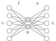

An item-based autoencoder: the column of the matrix is encoded into a short vector and decoded into ; the user-based one works in the same way for the rows .
I refer to a 2017 paper on how to apply autoencoders to recommender systems; two variants, user-based and item-based, and it is very good that both can be implemented and compared. In appearance they are very similar to each other: as a neural network, one encoder layer gives the vector representation and one decoder layer, but now they are nonlinear thanks to the activation function. Moreover, everything we said about the various kinds of autoencoders can be taken and applied here. In particular, the denoising autoencoder works quite well. It optimises this functional by the stochastic gradient method, but, choosing at random a pair from the transaction data, it does not simply take a gradient step: with some small probability, usually about 10 per cent, it spoils the original data. This is done so that, having trained on noisy data, it recovers code representations of the objects that are robust to noise. For them to be robust to noise, they must be trained on noisy data and reconstruct the vector representations well, in this case item-based, that is, the vector representations of our items, even if we deliberately introduce noise. In this way we train the autoencoder to work even under strong noise and to form good vector representations of the items. This method turned out to be quite successful, and here too there is a play with weight coefficients: a larger weight is given to the noisy data. Various options for assigning the weights were tried, and the optimum turned out to be this: we give one to the noisy data and 0.65 to the non-noisy. Comparing item-based and user-based led to the conclusion that item-based for some reason works better; this, of course, may depend on the particular problem and on the proportions of the matrix , whether we have more items or clients and which of them is sparser, that is, this recommendation may turn out not to be universal.
Additional data in matrix factorisations and autoencoders
Let us see how various additional information can be taken into account in matrix factorisations and autoencoders. This is a good way to fight the cold start problem. If we have only the matrix and a new item or a new client has appeared, the question arises to whom to recommend the new item and which items to recommend to the new client if there is no history. Only the presence of some additional information about clients and items saves us. A client does not come to us "empty": he has not yet bought anything in our online shop, but we have, for example, obtained some data about him somewhere, and we have a vector representation of the client who has come to us; we do not know him, as it were, but in fact we already know him a little. The same with items, goods: of course there are some descriptions of goods, verbal or vector ones, from some characteristics. So in real business there is in fact always additional information, some feature vector descriptions of both clients and items, and they can be used.
Definition (Additional data in MF and autoencoders). is the feature vector of the client ; is the feature vector of the item .
A predictive model with parameters :
Matrix factorisation: .
Neural network autoencoders with additional data:
The drawback: it is impossible to take and into account at once.
F. Strub et al. Hybrid recommender system based on autoencoders. 2017.
One can build, for example, linear models of this kind, which take into account not only the interest profile, the scalar product of and , as usual, we already understand that, but also add a linear model for both clients and items: in effect one bilinear and two linear models. In matrix representation we get this problem: , and are fixed matrices, our input data, and we build four matrices: , , , . Similarly one can use neural network autoencoders and take additional data, the matrices and , into account in the neural networks; additional parameters will appear, by which this model differs from the autoencoders on the previous slides. There is a small drawback: the matrix can be taken into account only in the user-based approach, and the matrix only in the item-based approach. How to take them into account at once? This particular model does not give that possibility. Matrix factorisation allows it, but autoencoders have a small snag here, connected with the structure of the data and the structure of the model: one cannot take both into account at once just as freely.
Factorisation machines
There is one more approach, implemented in a fairly popular open library for collaborative filtering that one can use; it is called libFM, factorization machines.
Definition (Additional data in linear and quadratic regression models). is the feature description vector of the pair .
Examples of features: for films, the text of the description, tags, actors; for music, genre, performer, tags; for events, the text of the description, geolocation, reviews; the one-hot encoding of the client ; the one-hot encoding of the item .
A linear regression model for (it does not describe links between clients and items):
A quadratic model: let us add interactions between features:
Let us represent the weights by a low-rank matrix factorisation: , :
- an adjustable number of parameters;
- if there are no additional features, we get LFM;
- it is tuned by SGD or ALS;
- the most powerful tool is the libFM library.
S. Rendle. Factorization machines with libFM. 2012.
It is based on our forming in some way a feature description vector at once for the pair "client–item": as soon as we have , we can form some vector description for the given pair. What can be in it? Some features of the item, some features of the client. If it is a matter of recommending films or music, one can use text descriptions, the texts of reviews, some substantive content. Or one can do something quite simple and use one-hot encoding: for each client a vector of dimension equal to the cardinality of the set of all clients, with a one in one place; we have, as it were, encoded by a binary vector that we are dealing with the given client. Clearly this is highly redundant, highly sparse information, but nevertheless it is a crude way of vector representation, albeit of very high dimension, for the client and for the item, and in the model it is a way of taking into account the specific properties of the client and the item. The linear regression model then looks like this: here is our vector representation of the pair of features, and the linear model is simply a linear combination of these features. But may be gigantic, especially if we use one-hot encoding, so the dimension has to be reduced somehow, and there are many different approaches. In particular, low-rank matrix factorisations can be inserted in different ways: the coefficients of the quadratic model , which may be a gigantic matrix, can be represented at once as a low-rank matrix factorisation , where is a matrix of substantially smaller size. Such a model, trained by the method of least squares, is what the libFM library builds, and it is fairly efficient. What is good about this method? Not only that it has a single, computationally efficient implementation, but also that in various special cases it passes into LFM, ALS or other matrix factorisation methods; non-negativity constraints can also be imposed. A fairly powerful tool of a fairly general form.
Hypergraph models
And finally I would like to tell about one more approach, about a general view of recommender systems altogether. A great deal of interesting work has been done here, and, as I said at the beginning, there are very many ways of taking into account the most diverse additional information.
Definition (Additional data representable as a (hyper)graph). is the vocabulary of attributes of clients (socio-demographic data, region, hobbies…); is the vocabulary of properties of items (the words in text items); is a finite set (vocabulary) of situational contexts; is a finite set (vocabulary) of moments of time.
Kinds of transaction data:
- : the client chose the item ;
- : the client has the attribute ;
- : the item has the property ;
- : the client trusts the client ;
- : the client tagged with the tag ;
- : the client chose the item in the situational context ;
- : the client chose the item in the context at the moment of time .
The input data of a recommender system as a multipartite (hyper)graph: clients , items , attributes of clients , properties of items , contexts , moments of time (slide).
Here is such a general view of the input data in recommender systems as a multipartite graph. Originally, classically, in the so-called 2D models there are users and items and interactions between them, a bipartite graph; that is the classics. Next we say that users can be described by some attributes; these are called attribute-aware approaches in recommender systems. Items too can be described by some feature vectors; this is content-aware: for example, our items are text documents, texts consist of words, and we get feature descriptions, for example TF-IDF or feature descriptions by word2vec or a topic model, that is, we begin to use vector representations. The scheme with four sets , , , is what we talked about a few slides ago, when we used vector feature descriptions of clients and items. But one can also use, for example, information about in what context the user makes his choice. He may watch a film alone, with friends, with family, with his girlfriend; these are all different contexts in which the preferences of one and the same person will be different; or he buys a film to give it to a friend. Taking these contexts into account is quite different from the point of view of the structure of the model: a non-pairwise interaction arises. Until now we have talked about pairwise interactions, and here the interaction is a triple one: the user chose the given item in the situational context , that is, a third set appears, of situational contexts, and it is added as the third element to the "user–item" pair. This is an interesting aspect: now the interactions are no longer only pairwise, and this is not even a graph but a hypergraph, where the edges are not only pairs but also triples, quadruples, in general some finite subsets of vertices. Or a structurally still more complex situation: the client chooses an item in a situational context at a moment of time ; one more set appears, moments of time, and the moment of time acts as the fourth participant of the transaction. That is, the original transactions may be pairs, triples and quadruples.
Definition (A multimodal hypergraph topic model). The general idea of graph embeddings and topic models: the observed edges are generated by similar vectors of vertices.
Training vectors of the form , embeddings: . For probabilistic topical embeddings, the EM algorithm; for general embeddings, stochastic gradient.
How are models to be built in this case? In fact there is nothing complicated: one simply has to take different kinds of additional data into account. I have written them as information about frequencies, how many times a client chose an item in a situational context and so on; the data may be binary, may be frequencies. For example, in terms of topic modelling there are no obstacles to writing out a probabilistic model of the realisation of such a pair, triple or quadruple. If we have information about the interaction of some two sets, for example and , we must use the topical profile of the element and the topical profile of the element . It does not matter what nature the elements forming the parts of the graph are: for any multipartite graph we can write out a probabilistic model using the maximum likelihood principle; we want to take triples or quadruples into account, no problem, additional factors simply appear in the probabilistic model. Everywhere the model can be written so as to determine topical profiles, interest profiles, for elements of any types, of any nature. For optimisation, if it is a topic model, we have a general theorem that allows any such problem to be solved, maximisation over normalised non-negative vectors, elements of simplices. If there are no constraints of non-negativity and normalisation on these vectors, methods of the stochastic gradient type can be used to optimise such functionals. In effect this is multi-criteria optimisation: we try to describe everything we see, all types of data, by the same vectors, and this leads to log-likelihood functionals appearing that we add with some coefficients. Such is a very general view of taking into account practically any additional information of a transactional nature in recommendation problems.
Evaluating the quality of recommendations
The precision and recall of recommendations
The last thing I would like to talk about is how the quality of recommendations is to be measured.
Definition (Measuring the quality of recommendations). RMSE, the accuracy of predicting ratings (as in the Netflix Prize):
The accuracy of prediction does not guarantee good recommendations.
are the first recommendations for the client ; are the true preferences of the client .
More adequate metrics of the quality of recommendations:
- , precision;
- , recall;
- measures of ranking quality: MAP, NDCG and others.
G. Shani, A. Gunawardana. Evaluating recommendation systems. 2011.
The functional used in the Netflix competition, as I have already said, is not a very fortunate one. If we make recommendations for living people and form lists of recommendations for them, we are forced to evaluate quality after all as in a ranking problem. The functionals we considered last time, when we studied the learning to rank problem, come to our aid: precision, recall and then all sorts of quality criteria of a ranked list, MAP, NDCG and so on; all this is used to measure the quality of recommendations.
Diversity, novelty, coverage and others
Definition (Multiple criteria in recommender systems).
- Diversity: the number of recommendations from different categories or the degree of difference of recommendations between the client's sessions.
- Novelty: how many of the recommendations are items new to the given client.
- Coverage: the share of items that have at least once been among the recommendations.
- Serendipity: the ability to guess unexpected, non-trivial preferences of clients.
- Bias (propensity): past recommendations influence the clients' choice, skewing subsequent recommendations.
One can optimise a linear combination of the criteria, or optimise one under constraints on the rest.
The matter does not end there: there is a whole heap more criteria one has to pay attention to if one wants to build good recommendations. How diverse the recommendations are, how often we offer something new to our users, whether we offer new items to anyone at all. I draw your attention to the fact that some of these criteria are important for users, for example diversity, novelty or serendipity, that is, the model's ability to guess non-trivial preferences of users, while such things as coverage are the business interest of the recommendation service: it must ensure that all items are offered to someone in one way or another, that there are no goods left that are offered to nobody, and this of course has to be taken into account separately in the criteria when building models. There is one more big problem with recommendations, the so-called filter bubbles, and connected with them is such a criterion as bias. There are big debates now about how to measure this bias, propensity, at all: how to ensure that past recommendations that the user accepted, making his choice, do not limit his choice in subsequent recommendations. This is a separate problem, but there is neither the time nor the opportunity to discuss it now.
Offline and online quality
Remark (Offline and online measurements of the quality of recommendations). A typical scheme of an experiment:
- we split the sample of sessions into training and test;
- we optimise an offline quality metric on the training part;
- we evaluate quality on the test part and choose a model;
- we deploy the model in the recommendation service;
- we conduct A/B testing and measure an online metric (money or the number of clicks).
Online and offline metrics may be weakly connected:
- offline it is not known what the user could have bought;
- offline it is not known what he would have bought without recommendations.
The conclusion from the experiments: to improve online quality, different aspects of quality have to be optimised offline.
And probably the last aspect: the online and offline quality of recommendations. Typically we build some recommendation model, it starts working, or even several models at once give recommendations to users, and we conduct A/B testing: some users are served by one model, some by another, and we then measure quality: whether the user really clicked on, bought, viewed, liked, rated the recommended item. In this way we get the possibility of comparing models on the basis of the real preferences of users. But that is when we have already launched the models into business processes, and that is, generally speaking, a risky undertaking: an unfortunate model may sink the profit and some other business indicators. The question: how, from historical data, to tune a good model that can be put into production without fear? There are various techniques here, and of course offline it is very hard to evaluate a recommendation model adequately, because it is not known what the user could have bought if we had given him such a recommendation, and it is not known what the user would have bought anyway, without any recommendations at all. If the user comes to us already with some intention, it is useless to recommend to him the item he will buy anyway: something else has to be recommended to him, that is, a cross-sell or an up-sell has to be made. There is no universal recipe here, but it is considered that the more diverse the criteria used offline, the better the model will then work online.
Summary
Remark (Summary). Latent models based on matrix factorisations and autoencoders have a number of advantages:
- the amount of stored data is reduced;
- external data are brought in for the "cold start";
- nonnegative and probabilistic embeddings are interpreted as vectors of "interests" or "topics";
- regularisers are easily added for multi-criteria optimisation of the quality of recommendations.
We have come to the end: collaborative filtering, recommender systems. We talked a little about correlation models, but mainly, of course, latent models are used now, which have a heap of different advantages and are able to take diverse additional data into account.
No comments yet
Be the first to share your thoughts.