August 30, 2026 · Lecture · LibreTimes
Machine Learning 2. Lecture 6. Learning to Rank
Contents
- What this lecture is about
- The problem setting of learning to rank
- Kinds of problem settings
- Examples of ranking problems
- The pointwise approach
- Ordinal regression
- The ordinal SVM
- The pairwise approach
- The pairwise criterion
- Ranking SVM
- RankNet
- From RankNet to LambdaRank
- Ranking in search engines
- The problem of ranking search results
- Ranking features
- TF-IDF and its probabilistic meaning
- Okapi BM25
- PageRank
- Ranking quality criteria
- Precision and recall
- Precision, average precision, MAP
- The share of defective pairs and AUC
- DCG and NDCG
- The pFound user behaviour model
- On the practice of big search
- The DSSM neural model
- The problem setting
- The neural encoder and word hashing
- The advantages of DSSM
- Summary
- Seminar
What this lecture is about
Today's lecture is about learning to rank, the very ranking that is used in search engines and in many other places. To begin with we will look at the general problem setting and the main approaches — there are three of them; then we will talk about search engines: how the problem is posed there, what is specific about it when you search for documents by queries; and a little about the neural network approach. Let us first work out in general terms how the ranking problem differs from regression and classification.
The problem setting of learning to rank
Kinds of problem settings
Definition (Learning to rank: kinds of problem settings). Given: , the training sample; , the relation " is better than " between objects of .
Find: a ranking function that recovers the correct order relation:
The criterion is constructed differently in three approaches:
- point-wise (an analogue of regression or classification);
- pair-wise (the quality of pairwise comparisons);
- list-wise (the quality of the ranked list).
The linear ranking model:
where is the feature vector of the object .
We have a training sample of objects, and what is given for these objects is not some , as in regression or classification, but the correct partial order relation: for some pairs of objects it is known that is "less" than — let us say " is better than ". This relation may not be given on all pairs, that is, it really is a partial order. The task is to find a ranking function, that is, a function of an object that we will train so that its values on pairs of objects are ordered in accordance with the given relation "better".
Accordingly, there are three different approaches to posing the optimisation problem. The pointwise one uses classification or regression to solve this problem. The pairwise one is in a sense the most natural for this problem, because it tries to formalise directly the number of wrong pairs, where the given relation is violated. And the listwise one is the approach that tries to assess how good the resulting ranked list, the search results, turns out to be. Usually we talk about search problems, where a list of found objects has to be formed and ranked correctly so that the user is satisfied with how the system presents the search results to them. This user satisfaction has to be formalised somehow, and there are many different approaches, which we will talk about.
The simplest ranking model is, naturally, linear. Just as in classification and regression, one has to begin with linear models: an object is characterised by numerical features , is a vector of the same dimension, and the ranking function is simply the inner product. It only remains to tune the weight vector so that this function reproduces the correct partial order relations on the given training sample.
Examples of ranking problems
Example (Examples of ranking applications). Ranking (Learning to Rank, LtR, L2R, LETOR) is needed wherever a system offers a person options for making a decision.
- ranking the results of a search engine;
- ranking recommendations to users (books, films, music, goods of an online shop, etc.);
- ranking the options for automatic query completion (Query Auto Completion, auto-suggest);
- ranking the possible answers in dialogue systems (Question Answering Systems);
- ranking the translation options for phrases in machine translation (Machine Translation).
Where is ranking used? One can say — everywhere there is a system that gives a person a choice among a large number of options. This is human–machine interaction: the system does not take control itself but gives the person the opportunity to choose among several best options. One can say it is a decision-making ideology in which the automatic system only evaluates and shows the person the best options, and the person chooses among them. Naturally, these are search engines; recommender systems that offer books, films, goods, music, anything — this too is forming a list of results. There are applications where ranking models are deeply integrated into other systems. For example, dialogue systems: inside the system, the answer to a question or remark of the chatbot's user is formed gradually, over several stages of weeding out possible answers; at each stage a ranking is done, and the ranked list is passed on to the next stage. The same in machine translation: inside the system several translation options may be formed over several stages, evaluated and the best chosen, and ranking is used there too. Or such a seemingly simple application as auto-suggest: when you start typing a query in a search engine, it already offers several options for completing it. This technology was first used in search engines and then spread to many other applications. We will talk separately about search results in search engines.
The pointwise approach
Ordinal regression
Let us start with a simple and rather old method called ordinal regression; it is an example of a pointwise method. We will go through the methods and see how the optimisation problems are posed, following the scheme point-wise, pair-wise, list-wise.
Definition (Ordinal regression (Ordinal Regression, OR)). Given: a sample , where .
Find: a ranking model with parameter vector and thresholds , , :
Criteria with a loss function decreasing in :
- the sum of losses over the two nearest thresholds:
- the sum of losses over all thresholds:
J. D. M. Rennie, N. Srebro. Loss functions for preference levels: regression with discrete ordered labels. IJCAI-2005.
Let us suppose that we do have after all. The setting is very similar to classification with one difference: a linear order relation is given on the finite set of classes, that is, it is an ordered set. For example, you rate objects on a five-point scale — 1, 2, 3, 4, 5 — and you know that there is an order relation between these ratings. How can a linear, or even a nonlinear, model be adapted to solve this problem? The ranking function gives a real numerical value on some axis, and it has to be matched with these ordered values, which have to be placed along the axis. We come to the idea that thresholds have to be set — as to saw a log into pieces one has to make cuts. These thresholds are part of the model and have to be determined. That is, we determine the parameter vector of the model and agree that if our ranking function gives a value in the range from to , the answer is .
If we output, for example, , our ranking function must fall into the strip between , the left boundary, and , the right one. We construct the loss function like this: if we fell into the strip, well done, the penalty is zero; if we fell to the left of the left boundary, we are penalised, and the penalty grows linearly; if to the right of the right one, also linearly. We know how to do such things: in classification it was the same — one has to introduce the notion of a margin and penalise violations. We introduce a decreasing function of the margin exactly as in classification, but, unlike classification, for each object we have two penalties, a penalty on the left and a penalty on the right, and the margin too comes out as a left and a right one.
The loss function for the sum over the two nearest thresholds, correct class (slide).
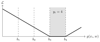
The sum of losses over the two nearest thresholds for an object with (with ): the penalty is zero while falls into the strip , and grows linearly on leaving it across either boundary.
But a question: if we gave such a wrong answer that, say, the correct answer is four and we said one, that is, we crossed the boundaries several times, we should probably be penalised even more strongly for that. Then the second, harsher variant of the loss function penalises large deviations more strongly, and this is right, because then more violations of the order relation arise. So instead of two terms for each object we introduce as many terms as we have thresholds, and we will penalise each crossing of a boundary. The result is a piecewise linear function: the further we move from the strip of the correct class, the more and more strongly we penalise.
The loss function for the sum over all thresholds, correct class (slide).
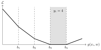
The sum of losses over all thresholds for an object with (with ): each threshold crossed adds its own penalty, so the slope grows with the distance from the correct strip.
I will not go further into how we solve this problem. You can probably guess: if we take the logistic loss function, it will be like logistic regression; if we take the SVM one, like SVM. By a small modification, introducing extra threshold parameters, we have managed to carry over the ideology of solving classification problems: there is a margin here and there is a functional that can be optimised, for example, by stochastic gradient.
Remark (A question: are the thresholds hyperparameters, or are they trained too?). Of course they are trained; they are not hyperparameters. The loss function is a function both of the thresholds and of the parameter vector of the ranking function : appears inside , and under . If we use, for example, stochastic gradient, there is no problem in differentiating with respect to both and . The idea here is that is simply more model parameters.
The ordinal SVM
Now let us see how SVM is adapted to this idea. Let me remind you what SVM is — a linear classifier; this slide is from last semester.
Definition (Reminder. SVM, the support vector machine). Given: , where , .
Find: a linear classification model , , .
The SVM training criterion:
where is the margin of the object .
The equivalent unconstrained minimisation problem:
For a linear two-class problem we build a separating hyperplane with direction vector and maximise the width of the separating strip; this is equivalent to unconstrained minimisation of the SVM loss function with a regulariser that in effect maximises the width of the separating strip. There is another name, ordinal classification, although in my view it differs very little from ordinal regression: it is practically the same method, but adapted from the very start to the SVM loss function.
Definition (The ordinal SVM (Support Vector Ordinal Regression, SVOR)). A special case of OR: the linear model , the sum over two thresholds, the loss function :
The equivalent quadratic programming problem:
Projections of objects of five classes onto the direction and the thresholds with margin strips (slide).
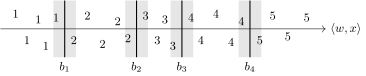
The ordinal SVM: objects of the classes are projected onto the direction ; the thresholds separate the classes, and the margin-width strips around the thresholds are where an object gets a penalty (schematic, our data).
Here is already the SVM problem setting for ordinal classification. The setting for ordinal regression was general, with an arbitrary loss function, and here we have in essence changed nothing except taking a particular loss function from SVM; I did this to show that the problem setting is analogous to SVM. Penalties are introduced for violating the left and right boundary for each threshold — these inequalities; the violations are non-negative, and we penalise them. The logic is exactly the same as it was in SVM.
Theorem (The SVOR dual problem). The dual problem ( for , for ):
The ranking model after solving the dual problem:
The advantages of SVOR are the same as those of SVM: the problem is convex and has a unique solution; nonlinear generalisations with kernels are possible; the solution is sparse and depends only on the support vectors.
Wei Chu, S. Sathiya Keerthi. Support vector ordinal regression. 2007.
Moreover, we write out the Karush–Kuhn–Tucker conditions and get the dual problem: it turns out quadratic with linear equality and inequality constraints, the problem is convex, has a unique solution and allows the inner product between objects to be replaced by a kernel. That is, all the bonuses that arise in SVM carry over here practically unchanged, the same ideology throughout. This means that we have in our hands a powerful tool for building not only linear ranking models but also nonlinear ones. As soon as we have replaced the inner product by a kernel, the line — the direction vector of the separating hyperplane — in the original space, just imagine, bends any way you like: a nonlinear kernel can provide the transition from linear ranking functions to nonlinear ones, enrich the parametric model and solve more complex problems with it. Ordinal classification is a typical example, and in fact a special case of ordinal regression, and an example of how the pointwise approach works.
The pairwise approach
The pairwise criterion
We move on to the next approach, the pairwise one. It is more interesting, used more often and, as a rule, works better in ranking problems, because it directly formalises the requirement not to violate the correct order relation.
Definition (The pairwise approach (pair-wise approach)). Given: , relations " is better than ".
Find: a ranking model with parameter vector .
The criterion of ranking quality over pairs:
where is a decreasing function of the pairwise margin :
- : RankSVM, Ranking SVM and others;
- : RankBoost;
- : RankNet.
R. Herbrich, T. Graepel, K. Obermayer. Support vector learning for ordinal regression. 1999. Y. Freund et al. An efficient boosting algorithm for combining preferences. 2003.
What do we do? We construct a pairwise margin. The ideology is again the same as in classification problems. For pairs where is better than — and the ranking function works so that larger is better — it would be correct for the value of on the object to be larger than on . If this is not so, it is an error, and we penalise it. The margin here, unlike in classification problems, is by definition the difference of the ranking function on two objects, while the logic stays the same: the smaller the margin, the worse, and a negative margin means an error. If we take a decreasing function of the margin, we get a continuous or even smooth criterion that can be optimised by any methods, including stochastic gradient. The main difference from classification problems is only that in classification we sum over all objects, while here we sum over all the pairs of objects for which the correct order relation is given in the training sample. The margins are pairwise rather than pointwise, and that is the whole difference.
When ranking problems began to arise — some time in the 2000s large search companies started using them actively — all the methods of classification theory, logistic regression, SVM, neural network approaches were carried over very quickly; literally within a year a pile of scientific papers came out. As soon as business produced such a need — to solve learning-to-rank problems — the scientific community practically closed this problem within a few years, simply by adapting a huge number of classification methods. Each such method was in effect another paper: RankSVM, RankBoost, RankNet.
Ranking SVM
Definition (Ranking SVM: the support vector machine for ranking). Given: , , relations .
Find: of the linear ranking model .
The criterion is the SVM problem for the pairwise approach:
where is the pairwise margin, .
The equivalent quadratic programming problem:
T. Joachims. Optimizing search engines using clickthrough data. 2002.
How is SVM adapted to the pairwise setting? Very simply. The same as we have already agreed, with the difference from the classical SVM that our margin is pairwise rather than pointwise. Likewise a linear ranking function, likewise the famous SVM loss function, the hinge loss. What is the difference from the classical one? Only that the variables denoting the penalties for violating the order relation between the -th and -th objects are now attached to pairs of objects. Otherwise it is the same classical SVM setting: we replaced the sum over objects by a sum over pairs of objects, and that is all. This setting is even closer to the classical SVM than the previous, pointwise one.
Remark (A question: where are the queries in these formulas?). After the lecture a student asked: the Ranking SVM formulas take no account of the fact that in search we have different queries, each with its own list of answers. The partial order relation is given not on all pairs but only on those that are comparable — in search, these are "query–document" pairs with one and the same query. The sum over pairs can be rewritten as a sum over all queries and over all pairs of documents returned in answer to the given query; other pairs simply do not enter it. I deliberately start with a more general setting, where I simply say that a partial order relation is given on pairs of objects: an order has to be recovered not only in search engines but in many other places too — for example, in recommender systems, where the orders are arranged differently. Search is just one particular application.
RankNet
Definition (RankNet: logistic regression for ranking). RankNet: the loss function , the model is a neural network or boosting:
The stochastic gradient method: at each iteration we choose a random pair :
A more efficient update: we choose a random object and a mini-batch of all the objects it is comparable with:
C. Burges et al. Learning to rank using gradient descent. 2005.
RankNet. Ideologically, the difference is that a different loss function was chosen — the logistic one, as in logistic regression. Again a linear model can be used, but even from the name one can guess that there is a hint: not only linear models are used but also neural networks; later boosting over trees began to be used, and that also works quite well. If we differentiate the loss function, that is, write out the gradient step of the stochastic gradient method, we get a quite obvious expression: we differentiate the loss function, and then differentiate the ranking function with respect to the parameters. I also draw your attention to the fact that is a parameter of the loss function, how sharply the losses change as the margin deviates from zero. In principle this is a redundant parametrisation in a linear model: plays the role of a factor on the parameter vector . But if the model is nonlinear, this parameter may be needed.
From RankNet to LambdaRank
Here I want to draw your attention to the fact that the pairwise method is very easily adapted to listwise problems: the transition from pair-wise to list-wise is very simple. I will now demonstrate it; it is described in a paper by Christopher Burges. If you want the state of the art in ranking, here is a paper from ten years ago; in effect the science of ranking as a whole was already closed in those years, and no fundamentally new approaches to learning to rank have appeared since then; only the models of ranking functions have become more complex.
Theorem (From the pairwise RankNet to the listwise LambdaRank). Let be a non-smooth functional of ranking quality; in particular, to compute it the list of objects may be ranked in decreasing order of the values . is the change in when are swapped in the list.
LambdaRank: multiplying the gradient by leads to approximate optimisation of the non-smooth functional :
- If , then changes in the direction of increasing .
- If , then changes in the direction of decreasing .
- The sum of these changes moves up or down the list.
- changes the size of the move while keeping its direction.
C. Burges. From RankNet to LambdaRank to LambdaMART: an overview. 2010.
There is one wonderful thing. When we start talking about information retrieval in more detail, we will understand that the quality of search results, the quality of a ranked list, can be measured in very different ways, but all these criteria are based on our having taken the objects and ordered them by the ranking function. The ordering operation makes all such criteria non-differentiable, and the stochastic gradient method, and gradient methods in general, are hard to apply: these functionals are as a rule piecewise constant, and they are very hard to approximate in any way. There is such an approach too, but I will show a trick that is much easier to implement. If you have any pairwise method for which you have written out the functional, differentiated it and are going to use stochastic gradient, then by a very simple trick it is adapted to optimising any listwise functionals, including non-smooth ones.
Suppose we have a non-smooth functional that assesses the ranking quality of our model and is based on computations over the ordered list: the objects are ranked in decreasing order of the value of , and at the top of the list are the objects that are the best from the model's point of view. We introduce the quantity , the change in the non-smooth functional if we hypothetically swapped the -th and -th objects in this list. It turns out, and this is proved in that paper, that if the gradient is multiplied by these changes, this leads to approximate optimisation of the non-smooth functional . That is, the pairwise method is very easily converted into a listwise one, and this is one of the main ideas used in practice.
The pairwise method is good in itself too. In one large search company it was said for a long time that it was the best choice, and despite all efforts they could not make a listwise method work better than the pairwise one; this story went on for several years, probably not without reason. Although another large search company always claimed that listwise methods worked better for them. With this I finish the general view: we have looked at all three approaches — point-wise, pair-wise and list-wise.
Ranking in search engines
The problem of ranking search results
Now let us talk in more detail about search engines specifically. What is specific about the problem of search results? The main question: what is ?
Definition (The problem of ranking search results). is the set of web pages or documents; is the set of queries; is the set of documents found for the query .
: the objects are "query, document" pairs: , , .
is an ordered set of ratings; are the relevance ratings given by assessors: the higher the rating , the more relevant the document to the query .
The correct order is defined only between documents found for one and the same query :
In search engines the user is given answers to a query, that is, the objects we compare with each other are "query–document" pairs: the query is what the user typed, the document is what the search engine found in response. The most interesting thing is that, since are "query, document" pairs, we can compare only those that have the same query: we have no right to compare documents where the queries differ, and our partial order relation is given only on pairs of documents returned in answer to one and the same query.
A search engine is usually built like this. First a very wide set is found roughly, for example the documents that contain the words of the query. This search is done with the so-called inverted index, which stores for each word the set of documents in which this word occurs; returning these sets and intersecting them is a fast operation, a purely technical problem solved extensively, through powerful hardware, large distributed storage and so on. That is a separate technological matter that we do not touch. And then begins the fight for ranking quality, because there may be millions of documents found in this dumb simple way, and one has to show the most relevant of them, and in screen-sized portions — 10–20 documents.
Another question: where does the training sample come from? We have understood how the objects are arranged — documents returned in answer to one and the same query — and only these can we compare. Who compares, and where do the ratings come from? Relevance ratings are done by special people called assessors. They are hired to do this rating work and are paid for each rating; in effect it is done in crowdsourcing mode. People make some tens of thousands of new ratings a month. Why are new ratings needed all the time? The internet constantly evolves and changes, and the training sample has to be replenished all the time. So the training sample is arranged like this: first, only documents relating to one and the same query are compared; second, the ratings on some point scale are given, as a rule, by live people, assessors. The sample turns out rather large, because in industrial systems the rating process can be put on stream.
Ranking features
Now — what features can be computed from a "query–document" pair.
Definition (Ranking features for search results). Text features:
- the words of the query occur in more often than usual;
- the words of the query occur in consecutively, as a phrase;
- the words of the query are in the headings or highlighted in ;
- the length of , the age of , the readability of , multimedia in .
Link features:
- the number of links to the document , to the site, to the domain;
- the number of links from thematically close documents;
- the number of useful links contained in the document .
Behavioural, click features:
- the document is clicked often (in total / for the query );
- the user stays on the document for a long time;
- after the document users rarely return to the search.
User features, for personalising search.
The first thing that comes to mind is text features: count how often the words of the query occur in the document. But variants arise at once: let us search up to lemmatisation, let us add synonyms, let us expand the query with similar queries, let us try to guess what the user meant and expand the query somehow, and so on. Another type of feature is how useful the document is from the point of view of links: how often other documents link to it, and how useful those other documents are. Here anti-spam measures have to be introduced too, because as soon as search engines appeared, spam documents linking to each other appeared at once, and this has to be counteracted; search engines counteract it successfully — without all these anti-spam filters we could not use them at all. And click factors: if a document is often clicked for the same or similar queries, the document is useful.
Three main types of features — text, link, click — but clearly dozens of different modifications can be devised for each. When machine learning was being introduced for the ranking problem in one search engine, first about 30 text features were devised, then link and click ones were quickly brought in, and the feature system grew very fast: first there were dozens, then hundreds, and in about eight years it grew to several thousand. And it became ever harder to devise new features that would not contain information already present in other features. At first devising a new ranking feature was a matter of a few days, but when 2000 features had accumulated, developing a new useful feature became a separate project of several person-months.
TF-IDF and its probabilistic meaning
Let us look in more detail at some classical features. The most often mentioned is TF-IDF, a measure of the relevance of a document to a query. A great deal has been said about this formula, but very little about what probabilistic model of text data stands behind it. And mathematicians, strictly speaking, have some objections to this probabilistic model; you will understand in a moment what they are.
Definition (TF-IDF, a measure of the relevance of a document to a query). (term frequency) is the number of occurrences of the word in the text ; (document frequency) is the number of documents containing ; is the number of documents in the collection .
is an estimate of the probability of meeting the word in a document; is an estimate of the probability of meeting it times;
is an estimate of the probability of meeting the words of the query in the document purely by chance.
The estimate of the relevance of the query to the document :
is the term frequency; is the inverted document frequency.
Term frequency is simply the number of occurrences of a term, or word, in the given text: an integer, how many times the given word occurred in the given document. Document frequency is the number of documents containing the given word, and is the number of documents. Capital letters will denote document frequencies, which count documents; small letters, term frequencies, which count words. If we consider that a uniform probability distribution is given on the documents, then is a frequency estimate of the probability of meeting the word in a document. Now let us estimate the probability of meeting the word in a document a given number of times — this probability raised to a power. And here a substitution of the probability space takes place. If we estimate frequencies on the set of documents, it is a probability space whose outcomes are documents. If we talk about word frequencies, we consider a probability space whose outcomes are words: the words of the dictionary appear in documents, and all this can be regarded as a single sequence of words cut up by documents, and on this sequence there is another probability space, for example the uniform distribution on all the words of the text collection. One has to understand that these two spaces are different: an estimate we computed as a document frequency we at once start using as a probability estimate in another probability space. At this moment we take an incorrect step — incorrect from the point of view of mathematics — but as a heuristic it is suitable in principle and works quite well.
Next we compute an estimate of the probability of meeting the words of the query in the document purely by chance. Consider: if you wrote some commonly used words in the query, words of general vocabulary, they really will occur often everywhere, and one has to take into account that this is most likely irrelevant: if a word occurs everywhere, the relevance estimate for it has to be lowered. We take such an estimate — simply the product over all the words of the query. If we get a small probability, this means that the words of the query occur in the document not by chance, that is, the document is relevant to the query. This is in fact similar to testing statistical hypotheses, the logic is the same: this quantity is the probability we would get if the words of the query and the words of the document were in no way related to each other, and the words of the query had wandered into the document purely by chance, simply because on average they are often used in all documents. If what is actually observed is much, much less probable than this formula predicts, the document is relevant to the query. For convenience this thing is put under a logarithm: the smaller the probability, the greater the relevance, so we take minus the logarithm. TF-IDF is a measure such that the higher its value, the higher the relevance. After taking the logarithm we got a sum over all the words of the query, and the term is exactly TF-IDF: term frequency, how many times the word occurred in the document, and ended up in the denominator, so it is the inverted document frequency.
Remark (A question: what is incorrect about it?). The incorrectness is not in any computational sense: two probability spaces are working at once, and few people pay attention to this. While we are told that is an estimate of the probability of meeting the word in a document, all is well: this is the space of documents with the uniform distribution. But when we start estimating the probability of meeting the word of the query times in the document, we have, strictly speaking, moved to another probability space — the sequences of words in a document — but carried over into it an estimate made in the space of documents. Strictly speaking, this step is incorrect, but as a heuristic it turned out to be quite workable, and this estimate is used in very many places in information retrieval.
Okapi BM25
This estimate has some shortcomings too, and the state of the art is considered to be its modification called best matching, Okapi BM25.
Definition (The Best Matching family of relevance measures (Okapi BM25)). A modification of TF-IDF:
- the growth of TF is bounded from above;
- TF is reduced for long documents;
- the IDF weight for frequent words becomes even smaller.
is the length of the document ; is the mean length of documents in the collection; controls how the document length is taken into account (usually ); limits the linear growth of TF (usually ); limits the strength of IDF (usually ).
S. Robertson, H. Zaragoza. The probabilistic relevance framework: BM25 and beyond. 2009.
There are three modifications. The first: we want to limit the growth of term frequency. There are documents in which for some reason a term is used anomalously often — the reasons may vary, including purely technical ones — and this growth has to be limited: not simply linear growth, but term frequency should be a function that saturates, so that it does not grow as the number of mentions of the term in the document grows further. The second: we would like to reduce the contribution of long documents: we want to compare short and long documents correctly, so that the results are adequate regardless of the length of the document — whether it has two words or two million. And the third: make IDF even smaller for frequent words. These modifications are shown in the formula. Here the length of the document is used in addition, and a function with parameters and : controls how the document length is taken into account, and limits the linear growth — TF was a linear function, simply equal to , and now it becomes a saturating function; appears in both the numerator and the denominator and controls how quickly the function stops growing as the frequency grows. The lower bound on IDF is the parameter . The added to the document frequency is often added in the original variant of TF-IDF too — a purely technical point, a slightly corrected frequency estimate so that a zero does not accidentally appear in the denominator. Later dozens of other modifications were devised, but we will not go into details. BM25 is in fact the best choice: if you are doing some kind of text search, TF-IDF can be used as a rough draft, but then throw it out and use BM25.
PageRank
The next type of feature in ranking search results is the classical link feature devised by Larry Page and Sergey Brin; it is called PageRank. There is a play on words here: on the one hand, Page is the surname of one of the authors, and on the other hand, it is the ranking of pages.
Definition (PageRank, the classical link feature). A document is the more important, the more links there are to from other documents , the more important the documents linking to , and the fewer other links these have.
The probability of visiting the page by clicking links at random:
is the set of documents linking to ; is the set of documents that links to; is the probability of continuing to click (damping factor); is the number of documents in the collection .
L. Page, S. Brin, R. Motwani, T. Winograd. The PageRank citation ranking: bringing order to the Web. 1998.
The idea is this: the importance of a document is properly estimated by how often other documents link to it. The principle: a document is the more important, the more links to it from other documents. But there are so-called link farms: some document lying around on the internet is in fact needed by spammers to raise the rating of some other documents. This must be taken into account in the downward direction: if the document has very many links, we must reduce the value of each of these links. The logic is this: a document is the more important, the more links to it from other documents, but we are interested in important documents, that is, links from documents have to be counted with different weights. And here the idea of a recursive definition arises: we want to determine the importance of a document, but in determining it we use estimates of the importance of other documents. We get a quantity that is defined through itself. The PageRank of a document is defined through the PageRanks of other documents — those that link to , that is, runs over the set — and if the document points to a set of documents , we push the cardinality of this set into the denominator. When will the value of a link be maximal? When is an important, valuable document and it has only one link — to ; then there is a one in the denominator, and an important document linking to strongly raises the importance of . If, however, links to a thousand other documents as well, we divide by a thousand, and the importance of such a link turns out smaller.
In fact such a model is equivalent to dropping our user into the link graph, where they start a random walk over the documents; then is the probability of reaching the document as a result of the random walk. A so-called damping factor is also introduced into this probabilistic model; it is usually set to 85 percent — the probability of continuing the walk. That is, with probability 15 percent you are picked up and thrown to a new random vertex of the link graph, and you start walking from there. The walking mechanism follows links with probability 85 percent and with probability 15 percent simply throws you to a random place, and such a walk model gives, by this formula, the probability of visiting the document . This probability is how important the document is: how often you will find yourself in it while walking over the huge link graph.
Ranking quality criteria
As the next step, let us deal with quality estimates. We need them, first, to understand how the quality of a list can be measured at all, and second — remember, we had the listwise approach, which needs criteria for evaluating the quality of a list.
Precision and recall
Definition (Evaluating search quality). Precision is the share of relevant among those retrieved; Recall is the share of retrieved among the relevant:
TP (true positive), retrieved relevant; FP (false positive), retrieved irrelevant; FN (false negative), relevant not retrieved; TN (true negative), must not be taken into account.
The problem: in "big search" FN and Recall are unknown.
Precision and recall (slide; an illustration from Wikipedia).
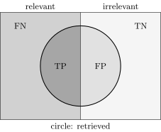
Precision is the share of relevant in the circle of retrieved; recall is the share of retrieved among all the relevant (the left half). The number TN is not used in search.
First, the classical measures of search quality, precision and recall; you have surely heard about this somewhere, I think I told it last semester, but let us recall it once more. The picture is taken from Wikipedia; it is very clear and shows very well what precision and recall are. I myself use a mnemonic rule, a mantra: precision is the share of relevant among the retrieved, and recall is the share of retrieved among the relevant. These two simple phrases illustrate the picture. All the relevant ones are in the left strip; everything you have retrieved is this circle. You of course need the green part of the circle to be as large as possible and the red part as small as possible. Precision — the share of relevant among the retrieved — shows the share of the green part in the circle, and recall — the share of retrieved among the relevant — shows the share of the green sector among all the relevant: how completely you have managed to find everything that was relevant.
Search differs from an ordinary two-class classification problem in that the true negatives — the grey zone, the irrelevant ones you have not retrieved — you are neither obliged nor supposed to find, and there may be arbitrarily many of them. This is the reason why true negatives are not used in these formulas at all. There may be millions, billions of objects in all, very few relevant ones among them, even fewer among what you have retrieved, and how many irrelevant ones you have not retrieved you do not care about at all, and the quality estimates must not depend on their number in any way. So of the four quantities listed, true negatives is the only one not used in these estimates. In classification, where there are sensitivity and specificity, the situation is a little different: there true negatives are used after all.
Precision, average precision, MAP
Now let us work with the results list. Our parametric trainable ranking function is used to form the search results: documents are ranked by its values. Denote by the -th document in decreasing order of the ranking function; the pair is in our original notation. We rank the documents found by the rough inverted index for the query in decreasing order of the values of the ranking function, and this is the whole difficulty: the function is trainable, it has parameters inside that have to be trained on a labelled sample, while the search results are formed by sorting by this function, and sorting is an operation that is not differentiable with respect to the parameters of the ranking function. Nevertheless it is precisely such things that we want to measure: how well the ranked list reflects our query, how relevant it is to it.
Definition (Precision, average precision, mean average precision). Let , be binary relevance; the ranking function being evaluated; the -th document in decreasing order of .
Precision is the share of relevant among the first :
Average Precision is the mean over the positions of the relevant :
Mean Average Precision is AP averaged over all queries:
First, precision, that same precision from the previous slide: the share of relevant among those retrieved. What are the retrieved ones? Let us agree: these are the first positions, the top of the ranked list. That is, precision contains the parameter and is a function of the query. What is it? The mean , where are the relevance ratings given by the assessors, that is, information from the training sample. We computed the mean relevance of the documents returned for the given query — that is exactly precision: we had very many documents, we took only the first of the ranked list — this is what we have retrieved — and we measure the quality of what was retrieved.
Now average precision. We want to get rid of , so we take the sum of the values , but only over the positions where there is a relevant document: if relevance is binary, or , multiplying by is exactly what reduces the number of terms — the sum only over those where . And mean average precision, which translates very badly into Russian, is when we also average over all queries. The MAP estimate is considered one of the classical ones, but still not a very good one. Where did go? I sum over here, but there must be some upper bound. As a rule is large enough, and when you sum over a long list it affects the estimate little, so I did not even bring it out as a parameter: little depends on it any more. But in precision matters a lot: if you measure only precision, you will in effect have to present a plot of precision against the position — against how many top positions of the search results you consider. Average precision removes this dependence on and makes the estimate more convenient, but not completely, because the question remains how much is; it has to be chosen in each problem, and this arbitrariness is built in too.
The share of defective pairs and AUC
How else can it be measured? One can measure the share of defective pairs. Here a small generalisation can be made already, and one can consider situations where the relevance ratings are arbitrary numbers and not only binary quantities.
Definition (The share of "defective pairs"). Let , be a numerical relevance rating; the ranking function being evaluated; the -th document in decreasing order of .
The share of order inversions among the first documents:
The link with Kendall's rank correlation coefficient :
The link with AUC (area under ROC-curve) in classification problems with two classes , :
The method stays the same: we consider the ranked search results — documents ranked by the function — and count the share of order inversions among the first documents. We sum over pairs of documents among the first — there are such pairs — and count the number of situations where is less than by our model , while the correct order relation between these documents, according to the relevance ratings, is the reverse. Such a pairwise measure is in fact related to a well-known statistical quantity, Kendall's rank correlation coefficient, and also to a quantity we went through last semester that is often used for evaluating classifiers, AUC. If you look at the definition of the area under the ROC curve, it too is defined through summing over pairs of objects and in effect also estimates the number of order inversions. But AUC works so that larger is better, while for the share of defective pairs smaller is better. So, up to normalisation and inverting the sign, AUC and the share of order inversions are the same thing; they differ by a normalising factor.
Remark (Maximising AUC is a binary ranking problem). For a classification model , the area under the ROC curve equals the share of correctly ordered pairs of objects of different classes:
so maximising AUC is a binary ranking problem with a pairwise criterion:
DCG and NDCG
What else can be devised to measure the quality of search results specifically in a more adequate way? We continue working in the situation where the relevance ratings are real.
Definition (DCG, Discounted Cumulative Gain). Let , be a numerical relevance rating; the ranking function being evaluated; the -th document in decreasing order of .
The discounted (weighted) sum of gains:
gives greater weight to relevant documents; gives greater weight to the beginning of the results.
The normalised discounted sum of gains:
is under ideal ranking.
We again consider the ranked search results, but now we want to take into account the user's logic: they look through the results from top to bottom and pay attention first of all to the documents at the beginning. So in the sum over the first positions there is a so-called discount factor that takes the order of the search results into account by an inverse logarithm: what is in the first line gets a weight much greater than what is in the second, third and so on — the weights of the lines in the ranked list decrease logarithmically. And how do we reward a relevant document having landed in this position? Here too there is an estimate that seems rather strange at first sight — 2 to the power : the relevance rating becomes very sensitive. If the rating is in points — 1, 2, 3, 4, 5, as assessors are usually asked to rate relevance on a five-point scale — then on a uniform point scale the gain grows exponentially: a document that got a five weighs twice as much as one that got a four. It is unclear where the binary logarithm came from, unclear where the power of two came from — these are heuristics. Clearly any increasing function of would do here, and any decreasing function of the position number there, but the information retrieval community settled on exactly this choice. It is a kind of social agreement among information retrieval specialists: everyone liked how this estimate works, and there are no other explanations of why gain and discount have exactly this form. But it took root, has been used for more than a decade, and is probably the most frequently used quantity for evaluating the quality of search results.
It is sometimes said that it is not very clear whether the numerical value of this quantity is large or small, how to characterise it quantitatively, so it is also normalised. is the DCG that would come out under ideal ranking: if among these we put the most relevant first, that is, ranked the documents not in decreasing order of but in decreasing order of itself. We compute the value under ideal ranking and divide by it — we get the normalised discounted sum of gains, which equals one only in the case of ideal ranking; it shows the degree of perfection of the ranking. NDCG is, one can say, the de facto standard in evaluating search results.
The pFound user behaviour model
But at some point one of the search companies devised a really cool measure, a user behaviour model called pFound — literally the probability that the user will find the document they need. How to measure the user's happiness — here is an attempt to measure exactly that.
Definition (pFound, a user behaviour model). Let , be relevance, an estimate of the probability of finding the answer in ; the ranking function being evaluated; the -th document in decreasing order of .
The probability of finding the answer in the first documents (by the law of total probability):
where is the probability of reaching the -th document:
is the probability of abandoning the search without an answer.
The difference here is that are relevance ratings in the interval , and one small addition: for the probabilistic model to be correct, the relevance ratings must in fact be estimates of the probability of finding the answer in the document . The relevance an assessor rates is, as a rule, a scale of 1, 2, 3, 4, 5, and it has to be converted into probability estimates. Clearly this is simple to do if you have somehow formed a sample in which you know for certain that the user clicked on such-and-such a document and remained satisfied, that is, found what they were looking for. That is, an additional auxiliary problem has to be solved — how to convert the assessors' ratings 1–5 into estimates of the probability of finding the answer in a document; its result is on the next slide. It is important that in this evaluation method be probabilistically interpretable quantities.
Then everything as before: we sort the documents in decreasing order of the ranking function and build a probabilistic model that estimates the probability of finding the answer in the first documents. The model is this: the user looks through the search results in order — the first document, the second, the third and so on. The probability of finding the answer in the first documents, by the law of total probability, depends, first, on the probability of finding the answer in each of the documents — this is why we convert the assessors' ratings into the probabilities — and second, on the probability of reaching the -th document. At the start it equals one, and then it begins to decrease: if you found the right answer in this position, you do not go further, you stop there. And is the probability of abandoning the search without having found the answer; usually it is 15 percent. In principle this too is a parameter of the evaluation method that can be tuned, but 15 percent is usually taken.
Example (The parameters of the pFound criterion).
- is the probability of abandoning the search without an answer;
- is the estimate of the probability of finding the answer in the document, computed from users' click data:
| Assessor's rating | ||
|---|---|---|
| 5 | Vital | 0.61 |
| 4 | Useful | 0.41 |
| 3 | Relevant+ | 0.14 |
| 2 | Relevant− | 0.07 |
| 1 | Not Relevant | 0.00 |
A. Gulin, P. Karpovich, D. Raskovalov, I. Segalovich. Optimising ranking algorithms by machine learning methods. ROMIP-2009 (in Russian).
Here is how the assessors' ratings were converted. They are on a five-point scale: a vital document is the highest relevance rating, a useful one rates a four, Relevant+ a three, Relevant− a two, and one is irrelevant. The probabilities were simply computed on a large sample: they estimated which last document users clicked on and, apparently, were satisfied with, and got an estimate of the probability of being satisfied on clicking a document rated by assessors. That is, it is a specially organised experiment on assessors and users; one can see how all this was done in the old paper.
On the practice of big search
Remark (On ranking search results (from my outdated information)).
- More than 50,000 new assessor ratings every month.
- More than 2000 features devised and tested over 8 years.
- The pair-wise approach is better than point-wise and list-wise.
- Alongside the assessors' data (explicit relevance feedback), larger but less reliable data on user behaviour (implicit relevance feedback) are used.
Technologies:
- MatrixNet: the ranking model is gradient boosting over ODT (oblivious decision trees);
- CatBoost: a freely available analogue of MatrixNet that works well with categorical features.
A few more points about big search. This information is somewhat outdated, about five years old, from the time when I worked on this; these are rough estimates. Assessors make about 50 thousand new ratings a month — really a large sample. These data are considered good and reliable, but there are still few of them, and one wants to bring in information about user clicks somehow. Ratings are of two types. Explicit relevance feedback — highly reliable but expensive ratings, relatively few of them; these are the assessors' data. And implicit relevance feedback — information about user behaviour, about how they click. There is a huge sea of these ratings, but they are not very reliable: if a user clicked, it does not yet mean the document is relevant — maybe they looked at it, did not like it, and started clicking on the next ones. One can use, for example, this consideration: the last article in the given search results that was clicked was most likely relevant. But on the whole clicks are an irresponsible thing: there are many of them, but they are unreliable. The question, of course, is how to combine both kinds of data — the assessors' ratings on a five-point scale and the huge number of unreliable user clicks.
What technologies are used to train ranking models? MatrixNet, gradient boosting over decision trees, very well made technically, very fast, capable of training on big data. CatBoost, a later technology: after several years of working with MatrixNet, all the best and most progressive things it had were put into CatBoost, and it was made open source. It is in fact not only for ranking but for any regression and classification problems with any loss functions — a freely available analogue of MatrixNet that works well with categorical features with a very large number of values. Roughly speaking, the user identifier can be put into it, and then we will gain by building more adequate relevance estimates for users with a long history.
The DSSM neural model
The problem setting
Now I would like to talk about where ranking went next. About five years ago people began gradually moving from ranking models on boosting — MatrixNet, then CatBoost — more and more to neural network models. One of the first neural networks they began to try is DSSM, the Deep Structured Semantic Model. In effect it is a simple model that internally learns a closeness function between a query and a document; both queries and documents are turned into vectors, that is, the model vectorises both queries and documents. It is somewhat similar to what happened in word2vec and FastText — recall the lecture before last. The main difference: this model is trained on user clicks — on implicit relevance feedback, that sea of not very reliable information that comes from users.
Definition (The problem setting for DSSM (Deep Structured Semantic Model)). Given: , the set of queries; , the set of clicked documents (clickthrough data).
Find: a probabilistic model of document relevance
is the cosine closeness of the embeddings , ; contains 4 random unclicked documents together with each clicked (negative sampling).
The criterion of maximum likelihood:
over the parameters of the encoder .
If we have a set of queries and a set of documents that were clicked in answer to a given query — it is called clickthrough data — this is our training sample, and we want to build a probabilistic model of document relevance. We want to estimate the conditional probability of how relevant a document is to the query : it is a distribution on the whole set of documents that are in principle returned for the query . One can say that the query went through the inverted index, which returned some number of documents — maybe a hundred, maybe a hundred million; on this set we introduce a discrete probability distribution defined through SoftMax over the closeness function between the query and the document. To each query and each document we would like to assign some vector representation — in our jargon, an embedding — and this probability is simply the closenesses renormalised through SoftMax: the closer the document to the query, the higher the probability. Through the exponential we guarantee the closeness values are non-negative and normalise them; this is not the first time you meet the SoftMax model — in effect it is a piece of multiclass logistic regression.
How are these embeddings built? We will train them, and we need a criterion. As is easy to guess, it is the maximum likelihood principle, but there is a nuance: we have what is called positive only. We know the clicked documents and can apparently consider them relevant, but where do we get a sample of irrelevant ones? The problem seems similar to two-class classification. What is ? I said: let us take the set of all the documents the inverted index returned. Of course this is not done, because the inverted index may return a hundred documents or a hundred million, depending on the query, and this set has to be limited somehow. So is formed in a limited way: for each clicked document about 4 unclicked ones are chosen in addition — a random subsample 4 times larger than the set . It is simply a way of normalising in SoftMax: we want to avoid having a hundred million documents in the SoftMax denominator — that would be impossible to compute. We have already met this idea when we talked about the vectorisation of texts and word2vec: recall SGNS, that very negative sampling, a way of avoiding an astronomically large number of terms in the denominator, so that one can still do stochastic gradient and differentiate with respect to the parameters of the closeness function, that is, with respect to the embeddings.
And one more heuristic in the maximum likelihood principle: the sum over all queries and over the documents from — unexpected, right? That is, the four random unclicked documents are used only to form the SoftMax denominator; in the maximum likelihood criterion we as it were give these documents zero weights — they are used only for normalisation, not as terms in the log-likelihood. Now about the model parameters. We have agreed how the closenesses of embeddings are converted into conditional probabilities, and we substitute them into the maximum likelihood criterion. And where are the parameters? The parameters are in effect the parameters of the neural network that generates the embeddings. There are many reminiscences of previous lectures here: we recalled word2vec, and now we will have to recall what an encoder and neural networks are. The parameters of the encoder that turns a document and a query into a vector representation are denoted .
The neural encoder and word hashing
Definition (The neural encoder in DSSM). A three-layer siamese neural network with parameters :
Word hashing: the document is represented by a vector of frequencies not of the words but of letter trigrams (the example is a made-up Russian word, «дармолюб»):
Po-Sen Huang et al. Learning deep structured semantic models for web search using clickthrough data. 2013.
Suddenly — a siamese neural network. What is that? It is a very simple concept; I did not even explain it separately on the slide. If you need to compare one document with another — and we are now building a trainable closeness function between documents and queries, with both documents and queries turned into vector representations — then a siamese neural network is a network, one and the same, that is used to vectorise both the query and the document. Why "siamese"? Siamese twins are two twins: one and the same network is used to vectorise two documents, but then these two vectorisations are combined in a common cosine closeness; trainable parameters can be built here too. The result is two twins, two identical networks joined at some part, and their result — two embeddings — is used further to compare the two documents, and the comparison estimate goes into the closeness function, into the probabilistic model, into the maximum likelihood principle. One can say that a siamese neural network is a way of training a closeness function, what is called metric learning, or distance learning.
The DSSM siamese network (slide; a figure from Huang et al.): identical towers for the query and the documents, the cosine closeness and the probabilities .
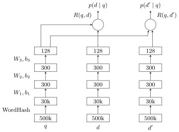
The DSSM siamese network: the query and the documents are vectorised by one and the same network (word hashing into up to 30 thousand letter trigrams, then fully connected layers 300, 300, 128); the cosine closeness of the embeddings gives through SoftMax.
Having understood this idea, let us look at how the neural network is actually arranged. It is rather simple: head-on, a fully connected three-layer neural network. A query arrives and is transformed by the three-layer network, a document is transformed by exactly the same network, then the formed vectors of the query and the document go into the closeness function — the cosine, in effect a normalised inner product — and from it the probability estimates are computed through SoftMax. The network for the query and for each document is in fact one and the same, with the same parameters — the matrices and the free terms .
What has been devised here that is non-traditional, tailored specifically to information retrieval and text analysis? We have already met such an idea when I mentioned FastText: the idea of splitting words into pieces. In this case the pieces are letter trigrams: what is vectorised is in fact not words but the letter trigrams of the original words. At the lower level there may be, for example, 500 thousand — half a million — words in the dictionary, and that is not yet the largest dictionary; there may be many millions. In search there are words with typos, neologisms, words someone has made up. If you vectorise whole words and a word has occurred for the very first time, its internal structure — what it consists of — may suggest some meanings. So the idea of splitting words into letter trigrams works very well when dictionaries are huge, when there are words with typos, new words, words similar to existing ones — people play with words and sometimes distort them deliberately so that some meanings can still be guessed. How can a neural network be taught to see these meanings in new words too? In this way. It is called word hashing: the originally huge dictionary of words is transformed into a far from huge dictionary of trigrams, about 30 thousand. Consider: if a language has about 30 letters, there are trigrams, about 30 thousand. We greatly reduce the number of tokens that are vectorised, for which we build embeddings, that is, the dimension of the parameter space shrinks at once. This hashing is also good in that it is insensitive to typos and can predict at least something for new words — for example, for that same «дармолюб». Then the vectors that word hashing gave us are fed to the input of a three-layer fully connected neural network, and it is this network that has to be trained on the huge sample of clickthrough data, the data on user clicks.
The advantages of DSSM
Remark (The advantages of DSSM).
- Thanks to word hashing:
- the number of vectors is reduced from 500k to 30k;
- words with similar spelling have close vectors;
- it becomes possible to handle new words,
- and also words with typos.
- Unlike other embeddings, which are trained without a teacher to reconstruct the data, DSSM is trained with a teacher, on big data on user clicks.
Let us discuss a little more what is good about this method. First, thanks to word hashing it is not the dimension but the number of vectors we look for that is reduced. Words with similar spelling can get close vectors: since the vector representation of a word is formed from the vector representations of letter trigrams, we get meaningful vector representations for words too. Robustness to typos arises, and it becomes possible to handle new words that have never occurred before: the word is new, but we split it into trigrams and manage to vectorise it. What else is good about DSSM? That it is trained precisely on click data — such a specialised model for search.
You will ask: and the assessors' data, are they not used here? In the initial version of DSSM they are not, but clearly one just has to build more complex models to take additional data into account. And click factors, link factors, other useful developments — can they be built into this model too? On the whole, yes, of course they can. The DSSM model was devised in 2013, and since then a huge number of modifications have appeared that extend it precisely in these directions: how to build in the simultaneous use of assessor and user data, how to take into account not only clicks but also link factors, and the variety of text factors developed over the years. And here, note, there is a very simple general scheme, and it has already turned out very successful: it really is great to compute vector representations of trigrams through word hashing. But this does not take into account all those developments — on synonyms, on how to take into account the positions of words within a text, markup: there may be words highlighted in the text, words in headings, in meta descriptions — all this is additional information that the simple DSSM model does not take into account. Later, more advanced models appeared that can take all this variety of information into account, combine it into a single model and train it in a similar way. And if it is a matter of using assessor and user data simultaneously, then two criteria are simply combined into one, and the parameters of one and the same model of vector representations are trained so as to take into account both implicit and explicit relevance feedback.
Summary
Remark (Summary).
- Ranking is a special class of machine learning problems: by the training sample it resembles classification, by the ranking functions it resembles regression.
- The criterion of ranking quality depends on the application; there is no best universal criterion.
- Three approaches: pointwise, pairwise, listwise. Theoretically the listwise one should be the best, but in practice the pairwise one worked better for a long time.
- Over time it becomes ever harder to create and improve ranking features; "big search" has moved to deep neural networks for ranking.
Tie-Yan Liu. Learning to rank for information retrieval. 2011. Hang Li. A short introduction to learning to rank. 2011. Fen Xia, Tie-Yan Liu, Jue Wang, Wensheng Zhang, Hang Li. Listwise approach to learning to rank: theory and algorithm. 2008.
To summarise briefly what we went through today. Ranking problems are a special class of machine learning problems, similar to classification and to regression. There are three ways of solving them — point-wise, pair-wise and list-wise; list-wise is an elaboration for optimising special ranking quality criteria more finely. There is no best universal criterion: in different problems one approach or another may be better. There are several good surveys on learning to rank; they are rather old, from 2011, and I have not managed to find equally thorough more recent surveys. I explain this by the fact that the ranking problem itself was conceptually closed already in those years: it arose at the beginning of the 2000s, by the beginning of the 2010s it was on the whole solved and closed, and after that it only remains to improve the models; the approaches are unlikely to change.
No comments yet
Be the first to share your thoughts.