August 30, 2026 · Lecture · LibreTimes
Machine Learning 2. Lecture 5. Topic Modelling
Contents
- What this lecture is about
- Probabilistic topic modelling
- The formulation of the problem
- Three interpretations of the problem
- Applications of topic modelling
- The maximum likelihood criterion
- Maximisation on unit simplices and ARTM
- The lemma on maximisation on simplices
- The ill-posedness of the problem and regularisation
- Additive regularisation of topic models (ARTM)
- The interpretation of the EM algorithm
- Regularisers: PLSA, LDA, background topics, decorrelation
- PLSA and LDA
- The Dirichlet distribution
- The maximum a posteriori probability for LDA
- From Bayesian learning to additive regularisation
- Background topics
- Decorrelating topics
- Multimodal topic models
- Modalities
- Unigrams and bigrams
- Multilingual models
- More regularisers
- Classifying documents
- Regression on texts
- Word co-occurrence: short texts
- Links between documents
- Topic hierarchies
- Summary
- Seminar
What this lecture is about
The topic of today's lecture is probabilistic topic models. In a sense this continues the ideology of the previous lectures: the vectorisation of an object that is complex from the outset, a natural language text. We have already talked about vectorisation when we considered models of the word2vec type, attention models, transformers. This is one more, alternative approach, not based on neural networks: a simpler technique. And it is a good occasion to talk about how diverse regularisers can be in machine learning, adding reasonable constraints to the original problem, which is possibly ill-posed. Today's lecture is about that too, and this, by and large, goes far beyond topic modelling: it is a much more general thing.
Probabilistic topic modelling
The formulation of the problem
Let us begin with the formulation of the problem. We will deal with data called a collection of text documents. There is a finite set, or vocabulary, of words; for generality we will call them terms, because sometimes not only words but also phrases are included in the vocabulary. I will say sometimes "words", sometimes "terms". And there is a finite set of documents; clearly, each document consists of words.
Definition (The problem of probabilistic topic modelling). Given: a collection of text documents as "bags of words":
- is the frequency of the word (term) in the document ;
- is how many topics we want to determine in the collection .
Find: a topical language model (the probability space ):
- : which words each topic consists of;
- : which topics each document consists of.
Criterion: the log-likelihood of the language model:
T. Hofmann. Probabilistic latent semantic indexing. ACM SIGIR, 1999.
The simplest topic models, to which we will confine ourselves today, are based on the bag-of-words hypothesis: we are interested not in the sequence of words but in how many times each term was used in the given document. That is, we pass at once to a frequency representation of the text, and is simply how many times the word occurred in the document . Be careful: frequency in text analysis is not as in physics; for us frequency will always be an integer quantity, we do not divide it by anything. Get used to this terminology.
What are we required to find? A probabilistic model of text generation: we want to model the conditional probability of words in a document. Dividing the frequency of a word in a document by the length of the document, we get a frequency estimate of this conditional probability; that is, we want to model our input data by this model. What is this model? A finite set of topics is introduced. About the topics we know nothing so far, except that there is a finite number of them: the cardinality of the set is known to us, we set it in advance. The total probability formula is written out, saying that a text is generated like this: a document has a probability distribution over topics, and to generate each word we must first generate a topic from this distribution, and then, knowing the distribution over words for this topic, generate a specific word from it. We get a two-stage process of data generation.
Why can be removed in ? This is one more hypothesis on which topic modelling is based, the conditional independence hypothesis. The total probability formula is always true, but an additional assumption is made that the process of generating words is connected only with the particular topic and the document does not influence it: as soon as the document has given us a topic for a word position, we have forgotten which document it was and consider that the word is generated by the topic alone. Had we not made this assumption, we would not have been able to write the topic model in this form, and you should recognise this form at once: it is simply the product of two matrices. Had we not removed , we would have the product of a dreadful three-dimensional tensor by a two-dimensional matrix, the model would have a monstrous number of parameters, and we simply could not determine them. Next we use the maximum likelihood principle to pose the optimisation problem.
Three interpretations of the problem
Let us interpret the formulation of the problem a little, to get a feel for which other machine learning problems it is connected with.
Remark (Three interpretations of the topic modelling problem).
- Soft biclustering of documents and words by topics.
- Matrix factorisation, low-rank and stochastic: , where .
- An autoencoder of documents into topical embeddings:
- the encoder ;
- the decoder ;
- the reconstruction problem: .
First, it is a clustering problem. Each topic is a distribution over words, documents are also distributions over words, that is, in distributions over words we are looking for some cluster structure: originally there were documents, and we want to find the centres of the clusters , that is, the columns of the matrix are in a sense clusters. Why is the clustering soft? Because we want to determine which clusters each document belongs to, and we move away from ordinary hard clustering, where each object belongs to exactly one cluster. For texts that is not very adequate: each document may contain a mixture of several topics, and we formalise this reasonable assumption by means of soft clustering.
On the other hand, it is a stochastic matrix factorisation. The original huge and sparse "words by documents" matrix, the matrix of our frequencies, is factorised into the product of two matrices of smaller dimension. The intermediate dimension is the number of topics, as a rule much smaller than the vocabulary and much smaller than the number of documents in the collection. Typical sizes: a hundred thousand words, a million documents, a hundred topics. Probability distributions live in these matrices: the columns of all three matrices are discrete probability distributions, that is, the sum of the elements in each column equals one and the columns are non-negative. Such matrix factorisations and such matrices are called stochastic.
The topic model as a stochastic matrix factorisation (slide).
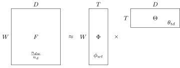
The topic model as a stochastic matrix factorisation : the "words × documents" frequency matrix of size is approximated by the product of matrices and ; the columns of all three matrices are discrete distributions.
And the third, very interesting interpretation. You now understand what autoencoders are; recall the lecture a couple of sessions ago. Each document can be understood as a distribution over words; that is our input. At the output of the encoder we have the topical representation of the document: the document is now represented by a vector over topics, and since there are far fewer topics than words, we have carried out a compression, built a vector representation of the document. But this vector representation differs from those we considered before in that there are constraints on it: it is a discrete probability distribution over topics, that is, normalisation and non-negativity. The decoder here is linear: in effect the matrix multiplies our representation from the left, and we get an approximation of the original frequency distribution of words in documents.
The topic model as an autoencoder (slide).
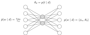
The topic model as an autoencoder: the encoder translates the frequency distribution of the document's words into the topical vector , and the linear decoder restores .
The interpretation through an autoencoder helps one realise that the roles of the matrices and are very asymmetric. In a matrix factorisation it seems that the two matrices play, as it were, symmetric roles; nothing of the kind. From the point of view of the autoencoder, the matrix is the encoded representations of the documents, what we get on the middle layer of the autoencoder, the topical vector representations of the documents, while is the matrix of parameters of both the encoder and the decoder. The reconstruction problem itself is posed as the same maximum likelihood, or, equivalently, as minimisation of the KL divergence: we want the outputs to approximate the inputs well, that is, the distributions of words in documents.
Applications of topic modelling
Example (Examples of applications of topic modelling).
- exploratory analysis of large text collections (how many topics there are in the collection and what they are about);
- finding topically similar documents;
- finding topical content in social media;
- detecting and tracking events in news streams;
- detecting consumption patterns in banking data;
- analysing nucleotide and amino acid sequences in bioinformatics.
J. Boyd-Graber, Yuening Hu, D. Mimno. Applications of topic models. 2017.
Where is this applied? Not only for clustering a large text collection: there is a mass of applications where the obtained vector representations of documents are used to solve other problems. For example, exploratory search in digital libraries: we begin to search for documents by meaning rather than by keywords, by these very vector representations. For the same purpose one can also use word2vec, FastText, BERT and much else. Finding topical content in social networks: we want, say, to do a sociological study, how much content there is on each topic; for this one first of all has to understand what topics there are at all, that is, to do an automatic clustering into topics. Topic models are good in that they allow this to be done unsupervised: no markup from experts, no you train on; at the input, text, at the output, topical representations. Analysis of news streams is also a very frequent application, when news stories have to be singled out and combined into topics. There are non-text applications too: in bioinformatics, when nucleotide sequences or proteins are analysed; the analysis of bank transactions, when a document is in effect the transactions of some client, and the transactions themselves play the role of words. Applying a topic model to these data, one can learn the patterns of consumer behaviour across the whole set of clients: in this case the topics are the economic, consumer behaviour of the bank's clients.
The maximum likelihood criterion
In a little more detail: where exactly this form of the maximum likelihood criterion came from. It is all very simple. As usual, we write out the probability density of the sample, then take the logarithm, and a sum of logarithms forms. Clearly we are entitled to do this only if we assume that the sample is independent; this is one more hypothesis of probabilistic topic modelling, but it is, by and large, universal for all probabilistic models in machine learning. Under the logarithm we get , that is, precisely the conditional probability being modelled; is in effect the length of the document, it does not depend on the parameters of the model, so we boldly strike it out as a constant. We get an optimisation problem, a mathematical programming problem. Note that the functional is essentially nonlinear: a bilinear model stands under the logarithm, with the constraints of non-negativity and normalisation: all columns of the matrices and are non-negative and sum to one.
Maximisation on unit simplices and ARTM
The lemma on maximisation on simplices
Now I want to tell you about a really neat general tool from mathematical programming with which one can crack any topic models like nuts, and not only topic models but any models whose parameters are discrete probability distributions.
Definition (Maximising a function on unit simplices). Let be a set of normalised non-negative vectors of various dimensions .
The problem of maximising a function on unit simplices:
K. V. Vorontsov. Rethinking probabilistic topic modeling from the point of view of classical non-Bayesian regularization. 2023.
The set of normalised non-negative vectors of various dimensions (slide).
Let us imagine that we need to maximise a certain functional that depends on a set of normalised non-negative vectors, and the vectors may even be of different lengths; that does not matter at all. In our case the matrices and give us a set of vectors: has as many columns as there are topics, and the size of each is the size of the vocabulary; has as many columns as there are documents, and the size of each is the number of topics. But in general there are many sophisticated, exotic topic models where, besides these matrices, some other parameters are defined that are also discrete probability distributions. And in such a general formulation the problem can be solved, and quite elegantly.
Lemma (On maximisation on simplices). The operation of normalising a vector: .
Let be continuously differentiable in . If is a vector of a local extremum of our problem and , then satisfies the system of equations
- The numerical solution of the system is the method of simple iterations.
- The vectors are discarded as degenerate solutions.
- The iterations resemble gradient optimisation , but they take the constraints into account and do not require choosing the step .
Let the function be continuously differentiable in all our vectors. Then this is a necessary condition for an extremum: if the vector is a vector of a local extremum and a certain strange condition holds, we will discuss it in a moment, then this vector must satisfy this system of equations. It is immediately clear how to solve such a system numerically: the method of simple iterations simply suggests itself, computing the left-hand side by computing the right-hand side head-on. For this to work, one naturally has to set an initial approximation for all our vectors.
Note how strongly this resembles ordinary gradient descent; I deliberately gave the formula of a gradient step as it would look if there were no constraints of normalisation and non-negativity. The difference is very small. First, our formula is multiplicative, and that one additive: plus has been replaced by multiplication, while the gradients computed are the same. Second, in our case, having taken a step and obtained a new value of the vector, we have to project it back onto the simplex, the set defined by the constraints of non-negativity and normalisation. This projection is carried out by the normalisation operation, which translates an arbitrary numerical vector into a vector of probabilities of the same dimension, and does so very simply: it sets all negative values to zero and then normalises. A similar operation you are used to is SoftMax, but the normalisation operation is simpler, there is no exponential here; the idea is very similar: both make from a vector a vector that can be interpreted as a discrete distribution. And the third difference from gradient descent: we have no gradient step at all, with which there are always problems, we always struggle to choose it. This came about thanks to this projection-normalisation operation. Otherwise it is very similar to a gradient method, and the main thing is that we need to compute only the partial derivatives of the functional with respect to the model parameters; we need not be able to do anything else.
Now about the condition. It says that if we compute the products standing under the normalisation, we do not get all zeros, that is, the denominator in the normalisation does not vanish. And if in practice it does vanish? Here informal agreements come into play. In principle one can derive a similar formula for this case too, but we will consider that in topic modelling it does not occur, and if it does occur, we will simply ignore the corresponding vectors and throw them out of the model: we will say that this is a wrong topic or a wrong document and refuse to model them. That is simpler and clearer.
How this lemma is proved I will not say: it is based on the Karush–Kuhn–Tucker conditions, which have already come up in our course more than once, and the proof is very simple: a head-on application of the KKT conditions. There one has to consider three cases for the sign of the dual variable, and the first case corresponds precisely to the condition we have stated here, that the denominator in the normalisation does not vanish; the other cases can be considered too, but, so as not to clutter the lemma, I did not put them into its conditions. We will use this nice identity simply as a tool for writing out the systems of equations that have to be solved.
The ill-posedness of the problem and regularisation
Now let us return to our problem and realise that the matrix factorisation problem is ill-posed.
Definition (Problems ill-posed in the sense of Hadamard). A problem is well-posed in the sense of Hadamard if its solution exists, is unique and is stable.
The matrix factorisation problem is ill-posed: if is a solution, then the stochastic are a solution too:
- , ;
- .
Regularisation is the completion of the definition of the solution by adding a criterion . Scalarisation of criteria: .
It is ill-posed in the sense of Hadamard because the solution is not unique. Indeed, if we have built a matrix factorisation , we can insert a square non-singular matrix here and its inverse here, and get one more solution, and in this way generate a whole family of solutions. Moreover, not all solutions giving a value of the functional close to the optimal one are linearly expressible through each other; that is one more large source of non-uniqueness. In short, our problem is underdetermined: the maximum likelihood criterion is not enough to obtain a unique solution.
This is not a drawback but, on the contrary, an advantage that can be extracted from this problem by imposing additional constraints, regularisation. If there are too many solutions, that is not bad but, on the contrary, good: it means we can require something else interesting of the solution and make it even better. So a fairly general approach arises: to our main criterion, the log-likelihood, we may well add another, and perhaps more than one, additional criterion. In the general case we say this: one can impose several additional requirements on the model and add all these criteria with some coefficients , which are called regularisation coefficients. This is not the first case in our course where two regularisers are applied to a model at once: recall linear models of classification and regression, elastic net, a sum of and regularisers with some coefficients. Topic modelling differs in having a very rich zoo of regularisers, and we will now go through them. This is probably the most interesting thing worth looking at here: how various requirements on the problem are formalised by means of regularisation.
Additive regularisation of topic models (ARTM)
Theorem (ARTM: additive regularisation of topic models). Maximising the log-likelihood with a regulariser:
The necessary condition for an extremum. A point of local extremum satisfies the system of equations
The EM algorithm is the solution of this system by the method of simple iteration.
K. V. Vorontsov. Additive regularization for topic models of text collections. Doklady Mathematics, 2014.
What we get by applying our lemma to such a functional is in effect the EM algorithm. Let me remind you: this is a system of equations describing the necessary condition for an extremum, but it is written in such a convenient form that it simply asks to be solved by the method of simple iterations. Our lemma writes out the system of equations in this form from the start, and we remember that these simple iterations are very much like gradient optimisation, only without a gradient step.
Proof. We apply the lemma to the log-likelihood with a regulariser :
where the auxiliary variables are singled out into separate equations and form the E-step in the iterative process.
How did this come about? In fact the derivation takes two lines: we apply our lemma to the log-likelihood with a regulariser, substitute into the formula and honestly differentiate. And here a little miracle happens: when we differentiate the logarithm, the topic model proper appears in the denominator, remains in the numerator, and then we multiply this by , and thanks to this the auxiliary variable appears. When we do the same for , we again single out the same variable, and it is set apart as the E-step. This theorem is a very powerful tool with which any topic models can be cracked like nuts, regardless of what the structure of the matrix factorisation is or how complex the regularisers used are: everything is easy, it is simply differentiated and normalised.
The interpretation of the EM algorithm
Remark (Properties of the EM algorithm for ARTM). The E-step is Bayes' formula:
The M-step is frequency estimates of conditional probabilities:
- is the frequency of the triple in the collection;
- is the frequency of the term in the topic ;
- is the frequency of the terms of the topic in the document ;
- is the frequency of the terms of the topic in the collection;
- and when there is no regulariser, .
The topic is degenerate and is excluded from the model (topic selection) if for all .
The document is degenerate, and the model cannot determine its topics, if for all .
This system is very interesting to interpret. The step at which the conditional probabilities of topics are computed for each word in each document gives us a very interesting estimate. The author of the text, when writing the word , was thinking about some topic, was trying to develop some topic, and estimating such conditional probabilities is in effect an attempt to recover what the author wanted to say. Such is the informal interpretation: which topics each word could belong to. We cannot assign it exactly, so we estimate a distribution over topics for each word. And the normalisation of the product is also interpreted wonderfully: it is nothing other than Bayes' formula; write out and through conditional probabilities, and you will notice it. An astonishing fact that came out by itself.
And if there were no regularisers at all, at the M-step you would get simply frequency estimates of conditional probabilities. Why so? Let us interpret : it is an estimate of the number of times the word in the document belonged to the topic . If we sum this estimate over , we get how many times in the whole collection the word belonged to the topic , and if we now normalise over words, that will be the conditional probability of the word in the topic. Exactly the same with the matrix . That is, very reasonable and clearly interpretable computational formulas.
Let us discuss a little that very condition: what we do when the denominator in the normalisation comes out zero, and how rarely this can happen. This is the degeneracy condition for a topic: if such a mess comes out for all the words of the vocabulary in a column of the matrix . is a counter, after all, and most likely it is fairly large; for the regulariser to make all the counters negative, the partial derivatives must become very large in absolute value and negative. This simply means that the regulariser has broken the model: it has been made excessively strong, and perhaps its coefficient simply has to be reduced a hundredfold, and all will be well. But sometimes this is useful: for example, it can do topic selection. You know what feature selection is; here regularisation can arrange a selection of topics, saying that thanks to your additional constraints this topic has turned out to be unnecessary. A good side effect. Similarly, if a column of the matrix is zeroed, then either the regularisation was applied too strongly, or the document is unsuitable: it consists of the wrong words or does not correspond at all to the subject matter of the collection, and the ability to detect such documents is also a good ability of the model.
Regularisers: PLSA, LDA, background topics, decorrelation
PLSA and LDA
Let us now consider examples of what regularisers there are.
Definition (PLSA and LDA as special cases of ARTM). PLSA (probabilistic latent semantic analysis): . The M-step is frequency estimates of conditional probabilities:
LDA (latent Dirichlet allocation):
The M-step is frequency estimates with offsets:
T. Hofmann. Probabilistic latent semantic indexing. SIGIR 1999. D. Blei, A. Ng, M. Jordan. Latent Dirichlet allocation. NIPS-2001, JMLR 2003.
The simplest case is when there is no regulariser, . In this case the M-step gives simply frequency estimates of conditional probabilities, as we have already reasoned looking at the formulas. This is a very simple model, and historically it was the first probabilistic topic model, invented by Thomas Hofmann in 1999, more than twenty years ago. It is called probabilistic latent semantic analysis, PLSA; it is simply the special case of a topic model without regularisation.
Another very well-known special case is latent Dirichlet allocation, LDA, and in it the regulariser is like this. Why it is like this we will now devote a few slides to, and we will figure out what the Dirichlet distribution has to do with it. Looking at the formula, you can probably already guess that it resembles cross-entropy, the maximum likelihood principle. It is indeed so: the formula says that the columns of the matrix should be similar, proportional to given distributions, only for some reason there is a minus one here; we will figure out in a moment where it came from. And in exactly the same way a constraint on the columns of the matrix : they should be similar to this distribution. The M-step comes out as a simple modification: let us differentiate this regulariser, which can be done in one's head: we differentiated with respect to , multiplied by , the logarithm differentiated into one divided by , cancelled, a constant remained. It turns out that this is the only regulariser that gives the frequency estimates of conditional probabilities simply a constant addition.
The Dirichlet distribution
Let us still figure out what the Dirichlet distribution has to do with it.
Definition (The Dirichlet distribution). The hypothesis. The column vectors and are generated by Dirichlet distributions, , :
What is the Dirichlet distribution in general? It is a distribution on an -dimensional simplex: it is able to generate normalised non-negative vectors, which in turn can serve as discrete probability distributions. The first thing to know about the Dirichlet distribution is that it is a distribution on a simplex. The second is that it can be either strongly concentrated or strongly sparse, and we are interested in the sparse case. What is a sparse Dirichlet distribution? It is a distribution that is mainly concentrated near the edges and vertices of the simplex: the middle is empty, and mainly vectors are generated in which most coordinates are close to zero, but never exactly equal to zero. This is one more important property of the Dirichlet distribution: it does sparsify, as it were, but not completely; zeros are forbidden here.
The parameter of the Dirichlet distribution is a vector. We generate the columns of the matrix from the Dirichlet distribution with parameter , that is, are vectors of dimension equal to the size of the vocabulary, and is also a vector of the same dimension; there are constraints on and on . Note also the parameter , which is simply the sum of all ; it, by the way, determines the variance of the Dirichlet distribution: the larger the sum of all our parameters, the more concentrated the distribution. Here it is shown on an example: all the coordinates of the vector equal ten, and we got a sharp peak in the centre of the simplex; this is the so-called symmetric Dirichlet distribution.
The density of the Dirichlet distribution with and (slide).
To get a further intuitive feel for how the Dirichlet distribution works, here are samples of three vectors each: each column is three vectors of dimension 10 on the simplex, that is, the sum of the coordinates always equals one, generated from the Dirichlet distribution. With a strongly sparse symmetric distribution, when the parameter equals one hundredth for all , one can see that in each vector some random single coordinate has a very large probability, and the others are very close to zero. If we increase the parameter of the distribution, we get more and more concentrated distributions. With we get the uniform distribution. Why uniform is easy to see from the formula: the power stands there, and if it is the power zero, it is simply a constant. The meaning of the normalising factor of the Dirichlet distribution also becomes clear: it is nothing other than the reciprocal of the volume of the simplex; with the uniform distribution the product turns into one, and we must divide by the volume of the simplex for the distribution to be normalised.
Samples of three 10-dimensional vectors with (slide).
Clearly, for topic models we are interested in the case where and are less than one, that is, the generation of precisely sparse distributions. It would be rather strange to see a document in which all the possible topics of the collection are present an equal number of times; sparsity is exactly what we need.
The maximum a posteriori probability for LDA
How can we add to the model the hypothesis that the columns of the matrix are generated from the Dirichlet distribution?
Definition (Maximising the posterior probability for the LDA model). The joint likelihood of the data and the model:
The regulariser is the logarithm of the prior distribution:
The M-step is smoothed or sparsed frequency estimates:
with , , smoothing; with , , weak sparsing; with , the prior distribution is uniform, PLSA.
The simplest way is the maximum a posteriori probability principle. We have to write out the joint likelihood of the data and the model. Its first part is exactly the likelihood of the sample, which we have already written before, but now it has to be multiplied by the Dirichlet prior distribution, a product over all columns of the matrix and over all columns of the matrix . We take logarithms and get exactly what I showed at the very beginning: that very simple regulariser. We differentiate it and get these modified frequency estimates, which are in fact either smoothed or sparsed depending on whether is greater or less than one. We agreed that we are interested in the case of less than one: then we get a negative addition. If the addition is positive, the frequency estimates are smoothed; if negative, we sparse them, and perhaps we even get a zero: in those cases where the counter was quite small, less than one, and also less than one, zeroing can occur.
From Bayesian learning to additive regularisation
But a question arises. From these formulas it does not by and large follow anywhere why we should impose non-negativity constraints on and . Clearly, the Dirichlet distribution is arranged this way and cannot be otherwise: there and are necessarily strictly positive. But, looking at the smoothing-sparsing formula in the M-step, we are puzzled: why, actually, can we not sparse more strongly, why does the Dirichlet distribution forbid it to us? In fact there are no grounds to consider that the columns of and are generated by a Dirichlet distribution. We can simply say: we have imposed a regulariser of this form and required that the columns of be similar to a given column ; why not? This will correspond to smoothing, and if is taken negative, it will correspond to sparsing. In such an approach, where we write out the regulariser right away and interpret it as cross-entropy, as an optimisation problem, we can forget about the Dirichlet distribution altogether, and this unties our hands: there are no longer constraints on the signs and magnitudes of the parameters and .
Remark (From Bayesian learning to additive regularisation). are the input data, the model parameters.
Bayesian inference of the posterior distribution (cumbersome, approximate) is done only for the sake of a point estimate of :
Maximisation of the posterior probability (MAP) gives a point estimate of directly, without inferring the Posterior:
Multi-criteria additive regularisation (ARTM) generalises MAP to any regularisers and their combinations:
Definition (The generalised LDA model (without constraints on the parameters)). Smoothing (, ) and sparsing (, ):
Smoothing the background topic with the general vocabulary of the language:
- : the topic is similar to the given ;
- : the general vocabulary is present in each document .
Smoothing by "white lists" (seed words, seed topics):
- : the terms from must be in ;
- : the topics from must be in .
Sparsing by "black lists":
- : the terms from must not be in ;
- : the topics from must not be in .
This is in fact a very useful tool: with such constraints one can say that the matrices and must have a certain structure. Let us see on an example what it can be.
Background topics
For example, we want to say that there are background topics. What are they? They are the words of the general vocabulary. One can hardly imagine a text in which absolutely all the words are terms of some subject areas. Perhaps some medical or mathematical texts look so mysterious that they seem to consist of terms alone, but no: there are still ordinary words there, words of the general vocabulary, and there may be quite a lot of them: perhaps half, or even 90 per cent. If we take a text and colour the different words by topics, we will see that a huge number of words remain, probably even the majority, that will stay white, uncoloured: they belong to no special subject topic; they are the general vocabulary.
Definition (Dividing topics into subject and background topics). Subject topics contain the terms of a subject area; , , , are sparse and substantially different.
Background topics contain the words of the general vocabulary; , , , are substantially different from zero.
The structure of the matrices and with subject (green frame) and background (red frame) topics (slide).
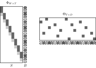
A schematic of the structure of the matrices (, subject topics; , the background one): for the subject topics the columns of are sparse and have different lexical kernels (conventionally, a diagonal band), and the rows of are sparse; for the background topic the column of and the row of are filled entirely.
The most natural way to model these linguistic considerations is to form background topics, that is, to say that in the matrix one or even several columns are responsible for the words of the general vocabulary, and in the matrix the rows corresponding to these topics are always filled, never sparse: in any natural language text the general vocabulary is necessarily present; otherwise it is some encoded, strange text, and we do not want to consider it. So to the background topics we must apply smoothing regularisation, even though we are talking about sparsing. Most topics we want to have in sparse form: we assume, for example, that each document has only a few subject topics, so the matrix looks sparse. And in the matrix we also assume sparsity: each topic has its own so-called semantic kernel, words that are in this topic but should not be in other topics, that is, they characterise only the given particular topic very well. The requirement that a semantic kernel different from the semantic kernels of other topics stand out in each topic I have conventionally depicted as such a diagonal dominance in the matrix , but of course in practice it will never look exactly like that; it is a convention in the picture, nothing more. Clearly, by means of smoothing-sparsing regularisation we can quite well say that some parts of these matrices should be sparsed and others smoothed: this is very easy to do by setting the coefficients and for blocks of these matrices negative in some places and positive in others, and in this way to formulate our wishes for the structure of the matrices and .
Decorrelating topics
And how do we decorrelate the columns, how do we say that the topics should be different? That is not hard: it is one more regulariser.
Definition (The topic decorrelation regulariser). The aim: to strengthen the difference of the topics; to single out in each topic a lexical kernel that distinguishes it from other topics; to help the general vocabulary pass into the background topics.
We minimise the covariances between the column vectors :
We substitute into the formulas of the M-step and get one more variant of sparsing, contrasting the rows of the matrix (the small probabilities in a row become still smaller):
Y. Tan, Z. Ou. Topic-weak-correlated latent Dirichlet allocation. 2010.
If we want to strengthen the difference of the topics and single out in each topic its lexical, semantic kernel, we must say this: for each pair of topics these topics should be close to orthogonal. This means that the scalar product of two columns of the matrix should be as small as possible, close to zero. Why are "close to zero" and the minimisation requirement one and the same? Because the vectors are non-negative, and the minimal value is attained when the columns are simply orthogonal to each other. But that is extremism, we do not need it: we expect that the topics will necessarily overlap in some words; there are polysemous words, homonyms, words that are necessarily used in different topics at once, and that is normal. We by no means require strict orthogonality; it is a soft constraint, saying that the topics should be different enough for each to have its own lexical kernel stand out. Then it remains to sum over all pairs of topics and put a minus, because all regularisers must be maximised.
Having written out such a regulariser, we must honestly differentiate it with respect to and substitute it into the formula of the M-step. First, we will see that this regulariser acts only on ; there is no in it, that is, only one of the two formulas is modified. The modification is a little frightening at first sight, but, first, there are no problems computing by it, and second, its interpretation becomes clear. We consider the rows of the matrix . Attention: the columns are probability distributions, while the rows are not normalised; a row shows in which topics the given word occurs at all. If one topic predominates in a row, this formula will lower the probabilities in all the other topics, and since there is a minus here, this regulariser is also a sparsing one: it decreases the small probabilities of the given word and perhaps even zeroes some of them. This is exactly what causes the contrasting, the lexical kernels will stand out: if some word has turned out to predominate in a certain topic, it decreases its probabilities in all the other topics. Our practice of solving a heap of different topic modelling problems shows that this is the most useful regulariser: it really improves quality in practically any problem by making the topics different.
Multimodal topic models
Modalities
One more type of problem, or rather a whole huge family of problems and a very important practical need, is modelling documents in which not only words are written. First, it is very useful to single out phrases, n-grams, terms, named entities and form a separate vocabulary from them: as a rule they are much more informative than single words; in a few slides I will show an example. But texts too contain not only words. There are metadescriptions: authors, time, sources and so on. Texts contain some objects: images or simply mentions of some entities that you want to consider separately for your applied problem. You have texts on astronomy, and you want to single out all the astronomical objects; texts on biology, zoology, botany: the names of plants and animals; texts on medicine: the names of drugs. A heap of examples where objects of a special kind are discussed that you want to model separately. Texts may have links to each other; that too is a non-text object. There is advertising on the internet, on pages or in search results. There are users who read these texts, download them, like them: as soon as a user has done something with a document, he has, as it were, written his identifier into this document. This, by the way, is a way of building a recommender system: if users leave their traces in the form of such tokens everywhere they have been, this can be regarded as an analogue of a text document.
Remark (A multimodal topic model). A topic can generate terms of different modalities: , , , , , , , , .
A multimodal topic model (slide): topics are described by distributions over words, n-grams, authors, moments of time, users, advertising banners, images and links.
All these entities, connected with the text in one way or another, can be modelled, and all of them described by distributions over topics: each topic will be described by a distribution over words, a distribution over authors, over moments of time, over users and so on. Such are the modern problems posed and solved on data from the internet, in digital libraries, in social networks: this diversity of entities is everywhere. The question seems a heavy one: how to model this? And the answer is very easy.
Theorem (Multimodal ARTM). is the vocabulary of tokens of the -th modality, . Maximising the sum of log-likelihoods with regularisation:
The EM algorithm is the method of simple iteration for the system of equations:
K. Vorontsov, O. Frei, M. Apishev et al. Non-Bayesian additive regularization for multimodal topic modeling of large collections. CIKM TM workshop, 2015.
For each such entity, we call them modalities, you write out its own log-likelihood and sum them with weights. We get, as it were, the same regularisation: there is a main modality, for example words, with its log-likelihood, and all the others go with some weight coefficients different from one; one can regard them as regularisers. Or one can consider that all modalities are in principle equal in rights and each has its own weight. Clearly, we will apply our main theorem in a flash to this new, slightly more complicated problem and again get the EM algorithm, a system of equations that differs from the previous one by only two additions. The first: for each modality the normalisation is done separately. We look for a matrix of its own for each modality, but the number of topics is the same, the topics are common to all modalities; one can picture one big matrix composed of blocks stacked on top of each other, but each block with its own normalisation. The second addition: we in effect multiply the token counters by the weight of the modality. For example, we have scientific papers as documents, say 5 thousand words in each, and on average 5 authors in each paper. If we consider words and authors on an equal footing, the authors will simply drown in this sea of words. The weight of a modality allows us to say: wow, authors are tokens that occur a thousand times more rarely than words; let us give them a weight of a thousand. Then we even them out in significance, and they will influence the formation of topics equally. Roughly speaking, the weight of a modality allows imbalances in the frequencies of tokens of different modalities to be removed.
This approach turned out to be very universal and powerful and covered a huge number of models. In the 2000s it was very fashionable to write scientific papers about models in which documents contain, besides words, some other entities: the entity-topic model, the citation-topic model, the author-topic model, the user-topic model and so on; practically every such case was treated as a separate paper. Looking at all this, we understood that all these are special cases of one general multimodal model.
Unigrams and bigrams
Example (The modalities of unigrams and bigrams). A collection of 1000 papers of the MMPR and IIP conferences, in Russian (the terms translated from Russian).
| Pattern recognition in bioinformatics: unigrams | bigrams | The theory of computational complexity: unigrams | bigrams |
|---|---|---|---|
| object | recognition problem | problem | separate sets |
| problem | set of motifs | set | finite set |
| set | system of masks | subset | condition of the problem |
| motif | secondary structure | condition | covering problem |
| solvability | protein structure | class | set cover |
| sample | recognition of secondary | solution | strong sense |
| mask | state of an object | finite | separating committee |
| recognition | training sample | number | minimal affine |
| informativeness | estimate of informativeness | affine | affine committee |
| state | set of objects | case | affine separating |
| pattern | solvability of the problem | covering | general position |
| system | solvability criterion | general | set of points |
| structure | informativeness of a motif | space | case of the problem |
| value | primary structure | scheme | general case |
| regularity | dead-end set | committee | MASC problem |
S. Stenin. Multigram additively regularized topic models. Master's thesis, MIPT, 2015 (in Russian).
This example, by the way, shows why it is very important to use not only, and not so much, words as bigrams. The collection taken is the proceedings of our conferences "Mathematical Methods for Pattern Recognition" and "Intellectualisation of Information Processing", in Russian, over a number of years, almost 1000 papers. I myself was the editor of the proceedings of these conferences, so I considered myself an expert on this collection: I knew all the authors by sight, knew who writes about what. I was curious how the topic model would deal with this collection and whether I, as an expert, would like the interpretation of the topics it singles out.
And this is what turned out. If topics are built on unigrams, that is, on single words, one can see that all the topics are about machine learning and pattern recognition: some recognition, some problem, objects, a sample; roughly what it is about is clear, but the specifics remain unclear. Only the words "mask" and "regularity" hinted to me who it might be. But when I looked at the same topic in bigrams, a single glance was enough to say what scientific school this is, who these people are that use such terms. The same came out with practically any topic. Another example: single words, set, class, space, problem, again something about data analysis; here too there were two words that gave a hint: "affine" and "committee". But in bigrams all the bigrams simply sang in chorus about who the authors of these papers are: these are easily recognisable terms. From this we concluded that building topic models on unigrams alone is uninteresting, not in the slightest. Bigrams are much more informative, but unfortunately in the literature on topic modelling probably 95 per cent of studies build models on single words. One should, of course, always take the trouble to preprocess the data: single out terms, phrases, named entities and so on; this turns out to be important.
Multilingual models
The next type of model, also a special case of multimodal ones, is multilingual models of parallel collections. Wikipedia comes to mind at once, a typical example of a multilingual collection. There are no exact translations there, they are rather retellings from one language into another, but nevertheless we can always consider that two articles connected with each other by an interwiki link have the same subject matter, that is, they have a common column in the matrix . This means that we can simply combine these documents, consider the words of different languages to be different modalities, and simply, dumbly, apply our multimodal approach. It turns out that this works really well: no pairwise alignments are needed, no bilingual dictionaries; all that is needed is the information that two documents are retellings of each other and share a common topical vector. This turns out to be enough to build absolutely remarkable models.
Example (The modalities of languages in multilingual models). 216 175 Russian–English pairs of Wikipedia articles, . The top 10 words and their frequencies in % (the Russian column of each topic is the model's Russian modality, kept as it is):
| Topic 68 | Topic 79 | ||||||
|---|---|---|---|---|---|---|---|
| research | 4.56 | институт | 6.03 | goals | 4.48 | матч | 6.02 |
| technology | 3.14 | университет | 3.35 | league | 3.99 | игрок | 5.56 |
| engineering | 2.63 | программа | 3.17 | club | 3.76 | сборная | 4.51 |
| institute | 2.37 | учебный | 2.75 | season | 3.49 | фк | 3.25 |
| science | 1.97 | технический | 2.70 | scored | 2.72 | против | 3.20 |
| program | 1.60 | технология | 2.30 | cup | 2.57 | клуб | 3.14 |
| education | 1.44 | научный | 1.76 | goal | 2.48 | футболист | 2.67 |
| campus | 1.43 | исследование | 1.67 | apps | 1.74 | гол | 2.65 |
| management | 1.38 | наука | 1.64 | debut | 1.69 | забивать | 2.53 |
| programs | 1.36 | образование | 1.47 | match | 1.67 | команда | 2.14 |
| Topic 88 | Topic 251 | ||||||
|---|---|---|---|---|---|---|---|
| opera | 7.36 | опера | 7.82 | windows | 8.00 | windows | 6.05 |
| conductor | 1.69 | оперный | 3.13 | microsoft | 4.03 | microsoft | 3.76 |
| orchestra | 1.14 | дирижер | 2.82 | server | 2.93 | версия | 1.86 |
| wagner | 0.97 | певец | 1.65 | software | 1.38 | приложение | 1.86 |
| soprano | 0.78 | певица | 1.51 | user | 1.03 | сервер | 1.63 |
| performance | 0.78 | театр | 1.14 | security | 0.92 | server | 1.54 |
| mozart | 0.74 | партия | 1.05 | mitchell | 0.82 | программный | 1.08 |
| sang | 0.70 | сопрано | 0.97 | oracle | 0.82 | пользователь | 1.04 |
| singing | 0.69 | вагнер | 0.90 | enterprise | 0.78 | обеспечение | 1.02 |
| operas | 0.68 | оркестр | 0.82 | users | 0.78 | система | 0.96 |
An assessor rated 396 topics out of 400 as well interpretable.
K. Vorontsov, O. Frei, M. Apishev, P. Romov, M. Suvorova. BigARTM: open source library for regularized multimodal topic modeling of large collections. AIST-2015.
We took a bilingual collection, Russian–English pairs of Wikipedia articles, there were more than two hundred thousand of them, and built a topic model with 400 topics. And lo and behold: topics singled themselves out, absolutely interpretable and, moreover, identical in both languages; among the top words in each topic one can even find simple translations of words from one language into the other. All this happened absolutely automatically: it was done by a bilingual, two-modal topic model that was given the collection as input, and there was no other markup. An assessor looked through all 400 topics by eye and said that he liked 396 of the 400: they are interpretable, roughly like these. Here is a topic about education and science, a topic about football, and a couple more examples: a topic about opera and theatre, about hardware and software. This is why we love topic modelling: it is a means of unsupervised learning that allows meanings to be singled out in large text collections without any human markup.
More regularisers
Next I will run through what other regularisers there can be and what can be done with them. In fact everything I am telling now consists of absolutely separate stories: if you have not understood one, you may well understand another. They are all exactly about our taking the formulas of the E-step and the M-step and substituting a particular regulariser into them, and we simply have to compute the additions; the most important thing is to formalise some regulariser.
Classifying documents
For example, one can solve classification problems on texts, and our multimodal approach already gives this possibility. Let us declare the classes one more modality: if a document has been assigned to some class, it is as if we had written the token of this class into this document as a word. A very simple way of encoding the original training sample for classification.
But with classes not everything is so simple. Sometimes we have information about which classes a document certainly belongs to, and that is the end of it: we do not know which other classes the document could belong to. Roughly the same happens in a recommender system, when we consider how users read documents: if we consider a user as a class, we see that he has read such-and-such documents, but do not know which others he could read; our task is precisely to build a model that will suggest this to him. And there are cases when we know for certain that a document does not belong to the other classes: this happens in text categorisation systems, where for each document it is known exactly which classes it belongs to, and it must not belong to all the others, and this requirement too has to be expressed somehow. We are talking about multiclass classification with overlapping classes, multi-class and multi-label, when each document may belong to many classes; this is precisely a typical situation for applying topic modelling, and text categorisation is one example of such a problem. If we write out the likelihood criterion, log-loss, for such a formulation, its first part corresponds to the information about which classes the document belongs to, and the second to which classes the document certainly does not belong to:
where is the set of classes of the document . The second part may or may not be there. If it is not there, the formulation of the problem falls exactly under the case of multimodality: a class is a modality. And if it is there, it has to be used as a separate regulariser: not only have we introduced the classes as a modality and automatically got the first half of the criterion, but we are obliged to introduce the information about non-membership into the overall criterion as a separate regulariser.
Regression on texts
One more interesting case is regression on texts, when from a text we want to predict some numerical quantity. Such problems also occur quite often. Suppose we want to use a linear regression model and take as the feature description that very topical vector of the document that the model gives us.
Definition (A regulariser for regression on texts). A linear regression model of documents :
The M-step for and the solution of the least-squares problem for :
This problem has two strategies of solution: one simple, the other correct. The simple one says: let us build a topic model with some LDA, get topical vectors for each document, in effect generate feature descriptions of the documents, and feed them separately to the input of some linear regression. Two ready-made black boxes one after the other: a simple engineering solution. But if the problem is to be solved correctly, we must say that we would like the topical vector representations of the documents to allow our main problem, the problem of regression on texts, to be solved well. So the regulariser must help us with this. The regulariser here is the method of least squares: we want to predict the numerical labels of the documents well with our linear regression model, and since take part here, this is in effect an additional requirement on our topics. We want to form the topics not just anyhow, not the way LDA happened to hand them to us, one of an infinite set of solutions, but to rotate these topics so that they are the most suitable for solving our particular least-squares problem.
Here one can recall autoencoders, which solve two problems at once: on the one hand, the reconstruction of the original sample of objects, on the other, an applied problem where the obtained vector representations of the objects are used as feature descriptions, for example for classification or regression. This scheme has come up, I think, for the third lecture in a row now, and that is very good, because it is a very correct, modern approach to problems: we simultaneously synthesise vector representations of the objects, make them good by means of reconstruction, topic modelling here being one of the possible ways of reconstruction, in effect an autoencoder, and at the same time use the vector representations of the objects to solve a particular problem.
We have the recipe: take the regulariser, differentiate it with respect to the model parameters, substitute into the formula of the M-step. What do we see? First, some intricate formula that is rather hard to interpret: it gives a regularising addition of either sign; it may turn out to be either smoothing or sparsing, some non-trivial correction of the topical vectors of the documents. And the second formula should be well familiar to you: it is simply the formula for the solution of the multivariate linear regression problem, giving the vector of coefficients , and the feature descriptions of the objects are the columns of the matrix ; the matrix here is the same as the "objects–features" matrix in ordinary multivariate linear regression. It works like this: with your topic modelling algorithm you run through the collection, one iteration of the EM algorithm is one pass over all the words in all the documents: for each word we compute the E-step and update the counters of the number of words in topics and topics in documents, a very simple one-pass implementation. After you have gone through the whole collection, the next approximation of the matrix has formed; now compute the pseudoinverse with this matrix, which will be the solution of the least-squares problem, the vector , and at the next iteration you will already use this vector in the M-step. The solution of the two problems is mixed in the iterative process: you refine the feature descriptions of the documents, then use them in the regression problem, which allows to be refined further, and so, iteration by iteration, you gradually converge to the feature descriptions, these vectors , turning out to be tailored not only to reconstructing the documents but also to solving the regression problem.
Where do formulations of regression problems on texts come from? For example, from a film review, predict what rating its author gave; from the description of a vacancy, predict the annual salary; from a review of some service, a restaurant, a hotel and so on, predict how useful it is, how many "helpful" votes this review will get. And probably the most notorious problem is playing the stock exchange, when the news stream is used to get signals for buying and selling certain financial instruments; this problem too can be posed as a forecasting problem on texts, and topic models used in it.
So we have counted five stories about regularisers of different kinds: smoothing and sparsing, background words can be singled out, that is one; decorrelation, making the topics different, that is two; modalities, all sorts of them, tags, classes, categories, named entities, languages, the multilingual model being a special case too, three; classification, the fourth case; regression, the fifth. And three more stories. The point is that this really is a powerful tool, and in the image and likeness of what happens in topic models one can construct the most diverse regularisers both for other problems on texts and for other problems in general: these are important examples of how fairly complex problems are solved with several criteria. The remaining three cases are links between words, links between documents and links between topics.
Remark (Regularisers for taking relations into account). biterm: word co-occurrence links ( is the frequency of a biterm):
relational: links between documents ( is the number of links):
hierarchy: links of parent topics with child subtopics , , the pseudodocument of the parent topic:
Word co-occurrence: short texts
The first case is very important. It came from the question: how to determine the topics of short texts? For example, tweets, the headlines of articles or news, literally a few words: how do we determine their subject matter? It turned out that the standard approaches work just abysmally: the matrix comes out extremely sparse, and the subject matter of short documents is determined very poorly. In effect one has to understand from a small number of words what the topics of these words are and add them up somehow. Any contrivances, perhaps combining some documents, perhaps using external information, building a topic model on Wikipedia and then going to study tweets with ready-made topics, none of this worked very well, and people searched for a long time for an approach to topic modelling of short texts. The good news is that in the end it was found, and it turned out to be the idea of using the co-occurrence of pairs of words. This is exactly the same idea that lies at the basis of word2vec, the model we considered the lecture before last, vector representations of words and graphs. A topic model can be built in exactly the same way, from data about paired co-occurrences of words, that is, in effect modelling now not documents but the links between words.
This is done very simply. For each word we compose a pseudodocument, the bag of all the contexts of this word. Suppose that in our whole collection the word occurs 10 000 times, and each of these ten thousand times it is in some sentence. We take this whole sentence as the context of the word, and from ten thousand sentences we compose a new document, a pseudodocument generated by the word , the set of all its contexts. Then instead of the counter of words in a document we use the counter of words in such a pseudodocument: counting how many times the word entered the pseudodocument of the word , we thereby count how many times the word occurred in the original collection in one context with the word , for example in the same sentence. We have in effect re-cut our collection: the original consisted of documents, and the new one consists of pseudodocuments corresponding to words; there are exactly as many of them as there are words, and each is the union of all the contexts of the given word . It turns out that if we take the collection re-cut in this way and build on it the most ordinary topic model, PLSA, LDA, regularised or unregularised, it no longer matters, we get topical vectors of documents that will in fact be topical vectors of words, since the documents correspond to words. And with such a model one can even solve the word analogy tasks that are the advertising examples for word2vec: "king minus queen equals man minus woman". It turns out that this came about not because some neural network model was built, but precisely because we took into account the pairwise links between words, their occurrence next to each other. After the re-cutting, the original documents can be forgotten for ever, the boundaries between documents have been erased, and we are interested only in how often words occur next to each other; we did the same when we built word2vec, where the problem was also posed as approximating paired co-occurrences of words. This way really does allow the topics of short texts to be determined well: the length of the document no longer matters to you; only the short local contexts of the words matter.
Links between documents
The second story is links between documents. If there are links, citations between documents, the set of documents is a graph with edges, and the problem is posed of taking this information into account when building a topic model. First, so that the links help determine the topics: if documents refer to each other, most likely they are from one and the same topic, and this information, additional to the word frequencies, may be useful for improving the topics. And on the other hand, such a model allows the most influential references to be identified. For example, we take a collection of scientific papers and ask ourselves: each paper has a list of references at the end, 30 items, 60 items; is it true that the paper relies substantially on all the cited papers? Of course not. There is a small number of papers on which the given paper relies substantially, and most likely these papers share some common subject matter with it. A topic model can be used to identify the most influential references.
Example (The influential references of the paper on the LDA model). As an example, the paper by D. Blei, A. Ng and M. Jordan on latent Dirichlet allocation is taken. The most influential for it by topical vectors turned out to be: T. Hofmann's paper on probabilistic latent semantic analysis, the PLSA model, which the authors criticised and for which they proposed a Bayesian regularisation; a paper on modelling heterogeneity with the Dirichlet distribution; and a paper by one of the co-authors, M. Jordan, an introduction to variational inference methods for graphical models, the Bayesian technique used to build LDA. All the other references, and there are several dozen of them, concern only minor aspects of this research.
Topic hierarchies
And the third story, last but not least, as they say. In fact this is a very important story in topic modelling, because very often the requirement is imposed on topics that there be some hierarchical structure: we want to single out in a text collection first large clusters-topics, then smaller ones, then smaller and smaller ones, that is, to divide topics into subtopics. If we talk about scientific papers, they divide into mathematics, physics, chemistry, biology, medicine, sociology, history and so on, two or three dozen such topics; then we want to divide each discipline into smaller ones, and so on, several levels. This story is in fact a very old one: library classifiers have been used since the 19th century. One can recall the Universal Decimal Classification (UDC), which has been used in libraries for more than a hundred years; it is built by a huge expert community, tens of thousands of people have put in effort to build this hierarchical system of classes, and nobody can now say exactly how many classes there are, but apparently of the order of a hundred thousand. Clearly, in the era of the internet and data analysis such library systems for classifying books and journals are becoming outdated; the means of search are completely different now. But the idea of building a hierarchical model of categorisation that would be understandable, so that from the root of the hierarchy one could reach any document in a few steps, find it and choose it, does not lose its relevance. Topic hierarchies are interesting, relevant and in demand. The problem is that probably hundreds of hierarchical models have been proposed in the literature, each more convoluted than the last. In our time we looked at all this, spat in disgust, and spent several years finally coming up with a simple, understandable and very effective hierarchical topic model.
Trees can be built in different ways: breadth-first, depth-first, layer by layer and so on. Here the strategy is this: we build topic models layer by layer, gradually increasing the number of topics; we simply build a sequence of models: the first with about 20 topics, the second with 100, the third with a thousand. Each time, building the next model, we must tie its topics to the parent ones, and it is desirable that these links be strongly sparse, that is, that each parent topic have a small number of children. When we build the model at some level, we assume that the model with the set of topics has already been built; these are the parent topics, topics; and are the subtopics, subtopics, and we must build a topic model where is greater than . How do we do this? As a regulariser we apply the requirement that the parent topics be approximated by a mixture of the child topics. The parent topic has already been built, the EM algorithm has already produced the counters for it, and we want to approximate this distribution of words in the parent topic by, in effect, a topic model of the child level.
If we look carefully at this formulation of the problem, it at once becomes clear that we are considering the parent topics as new documents, and the word counters in the parent topics as pseudodocuments into which we have simply thrown the distribution of words just obtained at the parent level. A very simple scheme results. We have built the parent topic model, taken its counters from the EM algorithm, in effect simply the columns of the matrix of the parent model, and begin to approximate them as new pseudodocuments, using the same maximum likelihood principle for this. That is, to the original collection we have simply added columns, as many as there were parent topics, and as counters we take , which are easily obtained from the EM algorithm. And the most astonishing thing: when we build the topic model of the child level, in the columns of the matrix corresponding to these newly added pseudodocuments we get absolutely free the links between parent and child topics, the conditional probabilities of the child topics given the parent one. The parent topic was in effect a document; it is now a column of the matrix , and the distribution in it over child topics is simply the links in our graph. Building each next level of the hierarchy is simply taking the matrix of the previous level, turning it into pseudodocuments and adding them to the collection; nothing else needs to be done.
Example (A topic hierarchy of a popular-science portal). On the collection of a popular-science portal a two-level hierarchy has been built: 10 top-level topics and about 50 topics of the next level; the edges of the graph are the probabilities from the matrix of the child model. For display the topics are named by their three most frequent words. So that topics similar in meaning stand side by side, the topics of each level are lined up in a chain by solving the travelling salesman problem on the pairwise distances between the columns of the matrix . The matrix of links is sparse but defines "many-to-many" relations, so among the child topics there are interdisciplinary ones, at the junction of several parents.
There are still a couple of minutes to explain what a topic spectrum is; this too is a rather amusing separate little problem. When we display topics for a person to look at, we first have to learn to name them somehow; here it is done in the simple way, the three top words in each topic. Clearly, how to name a topic properly is a separate problem, but the meaning of the topics is on the whole clear even after this. And then the problem is this: to place topics similar in meaning side by side. Topics are columns of the matrix ; we can compute the pairwise distances between them, that is, how close each topic is to every other, and pose the problem of lining up all the topics in one chain so that the distances between neighbouring topics are minimal. What problem is this? The travelling salesman problem: one has to go round all the cities so as to visit each once and wear out the minimal number of boots, that is, travel the minimal distance; and here the distances are measured between topics. There are ready-made algorithms for it, and with them the topics can be lined up so that they group side by side by meaning; this could be done for the child topics too. And it is amusing: some topics have several parents; one can see points of intersection, topics, as it were, at the junction of several parent topics. Since there is no strict constraint on the matrix of links that it define a tree, this matrix usually comes out well sparse but defines "many-to-many" relations between parent and child topics, and such interdisciplinary topics come out quite often.
Remark (A question: why some topics are present both among the parents and among the children). From the distribution of words in a topic, a column of the matrix , only the three top, most frequent words have been selected for display, and in principle they could quite well overlap in different topics and even coincide completely. There is nothing terrible in this: all the other words of the topic are simply not shown, and hundreds of words may have non-zero probabilities. This is rather a complaint against the simplest and not the most successful way of naming topics automatically by their three most frequent words; forming proper headings for topics is a separate, very interesting problem.
Summary
Remark (Summary).
- Topic modelling has three interpretations: soft clustering of texts; an autoencoder forming non-negative normalised vector representations of documents, interpretable in topics; stochastic matrix factorisation.
- The best-known models are PLSA [1999] and LDA [2001]. The problem is the inconveniences of Bayesian learning.
- Additive regularisation ARTM is multi-criteria optimisation with the possibility of combining models and building a model with given properties. The problem is choosing the regularisation coefficients.
- The lemma on maximisation on unit simplices radically simplifies both the theory and the practice of topic modelling.
K. V. Vorontsov. Probabilistic topic modeling: the ARTM regularization theory and the BigARTM open-source library. 2025 (in Russian).
Let us sum up. First, what topic modelling is: three interpretations. On the one hand, it is soft clustering of texts; on the other, an autoencoder able to form non-negative normalised vector representations of documents, interpretable in topics; and the third interpretation is stochastic matrix factorisation. Usually, when topic modelling is mentioned, LDA is what is used in practice, but I hope I have shown you that LDA is an outdated model twenty years old, which does not solve the problem of non-uniqueness, and that problem has to be solved with additional criteria, regularisers.
And another thing. If you look at the literature on topic modelling, you will notice that practically all topic models are built with the mathematical formalism of Bayesian inference. What I have shown you today is an optimisation approach, classical non-Bayesian regularisation, and this approach is radically simpler: you need be able to do nothing except differentiate criteria with respect to the model parameters, which is no harder than gradient methods. For some reason topic modelling uses precisely Bayesian inference, whose main purpose is in fact to obtain a distribution over the model parameters: not only to produce the matrices and , but also to say for each element of these matrices what distribution it comes from, most often the Dirichlet distribution. But the irony is that this richer information about the distributions in the matrices and is in reality never used by anyone. Bayesian inference in topic modelling is, in my view, simply using a sledgehammer to crack a nut: you have obtained a distribution over the model parameters and then immediately turned it into a point estimate, because for practice what is needed is precisely the matrices and , not estimates of their posterior distributions. The theory of topic modelling became simpler as soon as Bayesian regularisation was replaced by ordinary classical regularisation, and everything became much simpler; that is what I have told you about today.
And this lemma, or theorem, about how to do maximisation on simplices: frankly, we worked on topic models for some eight years, read more than a few hundred papers, and for some reason nobody did it this way, although it is the most natural and the simplest thing that can be used for topic modelling. Everyone overlooked it, although the fact is a completely textbook one; I do not know why it turned out so; science develops in strange ways. When you work on something for a long time, some eight years, you find ways of doing everything radically more simply than everyone else does.
No comments yet
Be the first to share your thoughts.