August 30, 2026 · Lecture · LibreTimes
Machine Learning 2. Lecture 4. Attention Models and Transformers
Contents
- What this lecture is about
- Sequence processing problems
- A reminder: the recurrent network
- A recurrent network for synthesising sequences (seq2seq)
- A recurrent network with an attention model
- Applied problems
- Interpretability: the attention matrix
- Varieties of attention models
- Similarity functions and the "query–key–value" model
- The attention formula and self-attention
- Multi-head attention
- Hierarchical attention
- The graph attention model GAT
- Transformers
- The transformer for machine translation
- The architecture of the transformer encoder
- Positional encoding
- The architecture of the transformer decoder
- Criteria for training and evaluating machine translation
- The transformer encoder BERT
- The BERT model
- Criteria for training BERT: MLM and NSP
- Fine-tuning and model sizes
- Summary
- Seminar
What this lecture is about
Today we will consider attention models, transformers and sequence processing. Attention models and transformers are precisely the models that made a revolution in machine translation, when we solve sequence to sequence problems: we translate a sequence into a sequence. A sequence of words in one language has to be translated into a sequence of words in another language, and the translation must be meaningful and such that a person likes it. Let us see how this miracle happened and what further changes and generalisations of these models appeared.
Sequence processing problems
A reminder: the recurrent network
Let us begin by recalling recurrent neural networks, which we have already had.
Definition (A reminder. The recurrent network (RNN)). Given: , a training sequence of vectors, .
Find: the parameters of a two-layer network in which is the hidden state vector at the moments , is the output vector (possibly ), :
The criterion for training the network:
Limitations:
- the lengths of the input and output signals must coincide;
- looking ahead is impossible;
- it does not suit many problems (MT, QA and others).
We have a sequence of input vectors; we denote the moment of time by , and each moment of time corresponds to some output vector or scalar . We assume that at each moment of time the network has a certain hidden state, which we encode by the vector . All three, , and , are vectors, generally speaking in different spaces of different dimensions. A recurrent neural network is simply a two-layer network: the first layer takes as input the current value and the previous value of the hidden state and forms from them the hidden state vector for the current moment of time; the second layer makes from this vector the predicted quantity . That is, it is assumed that the information contained in is enough to make a prediction.
A recurrent network and its unfolding in time (slide).
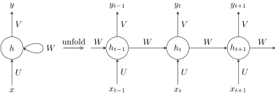
A recurrent network with hidden state and its representation unfolded in time (unfolding): one and the same matrices , , are applied at each moment of time.
It is often depicted like this, and the little loop shows that the network uses its previous state at each iteration. Sometimes an unfolding is done, this picture is unrolled into a sequence in time, but one has to understand that then one and the same network sits in each little circle, the same parameters: , , are matrices of weights, and here they are the same everywhere. To train such a recurrent network one uses, as usual, a functional that is a sum over all objects, in this case over all moments of time, of some loss function. Here we do not even say which one: whether you are solving a classification problem, a regression problem or something else, if you can characterise the losses from the answer at each moment of time by a smooth function, you formalise this as a function , depending on what problem you are solving. The architecture stays the same for a wide class of problems.
What is the drawback of this approach? That the lengths of the input and output sequences are equal: there is one and only one for each . For example, for the machine translation problem such a formalisation does not suit, because one and the same phrase can be said in different languages with a different number of words. One more drawback is that we keep running forward, a recurrent process in the strict sense of the word. But if we do, for example, machine translation, we usually listen to the phrase a little ahead after all; simultaneous interpreters always work that way. It is desirable, of course, to have a whole sentence and then translate it, that is, one has to look ahead. The whole input sequence has to be split into some pieces, sentences in natural language or something else in other applied problems, but there is some natural way of splitting the input sequence into pieces, and in each piece you are entitled to consider the input piece as a whole. This model does not allow that.
A recurrent network for synthesising sequences (seq2seq)
So generalisations appeared that are called sequence to sequence: there is a set of input sequences, a set of output ones, and each input sequence and the output sequence corresponding to it may be of different lengths.
Definition (A recurrent network for synthesising sequences (seq2seq)). is the input sequence; the output sequence; encodes all the information about for synthesising :
Limitations:
- remembers the end of the sequence better than the beginning;
- the larger , the harder it is to pack all the information into ;
- vanishing/exploding gradients will have to be controlled;
- an RNN is hard to parallelise.
Here is the length of the input sequence and the length of the output one. Keep the machine translation problem in mind all the time: I am considering one input and one output sequence, that is, I have introduced notation for one separate sentence in the input language, , and a sentence in the output language, . This is useful in order to interpret what is happening correctly from the start; had I introduced notation for the whole sample of sentences, it would have been more cumbersome. But remember that is only one small input sequence, one sentence, while in fact we have a huge collection of documents.
The idea is for the hidden vector to encode information not about one current word but about the whole sentence the network has read. How can this be generalised from the recurrent network model? I no longer go down to the level of matrices: an activation function of "matrix times vector" is a linear layer of neurons, and I simply write a function , an analogue of the first layer, which gets as input , an input element of the sequence, and , the state at the previous word. This is how the input sequence is processed. And the output one? The idea is that one recurrent network works over the input sequence, and a second recurrent network generates the output sequence element by element, word by word. A similar structure is used for generation, but the news is that, generating the output, we have to keep glancing at the hidden state that reflects the whole input sequence. Where do we get this from? It is the hidden vector that arises at the last element, when we have looked through the whole input sequence, that is, at the last word of the sentence we are going to translate. This must absorb all the necessary information from the input sequence in order to begin generating the output one.
The encoder–decoder architecture (slide).
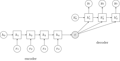
The "encoder–decoder" architecture: the input sequence is folded into a vector of fixed dimension, and the decoder unfolds it into the output sequence.
We get the encoder–decoder architecture: an input sequence of arbitrary length is transformed into a certain vector of fixed dimension, which the decoder then unfolds into the output sequence with a recurrent network. A technical question: at what moment should generation stop? It is solved relatively simply: at the end of each sentence, both input and output, there is a special end-of-sequence token, and this token, on a par with all the others, must be able to be generated by the decoder of the output sequence. No special constraint on the length of the output sequence is introduced, and this is exactly what allows machine translation to be done or other problems to be solved where the lengths of the input and output sequences need not coincide.
What are the drawbacks of this approach? First, as the length of the input sequence grows, the current state that comes out at the end keeps less and less information about the beginning of the sequence. But when we begin to generate the output sequence, its very first words, if we are talking about machine translation, must be connected somehow with the first words of the input sequence. This is in no way built into the architecture of the model: to translate each word, we have to look at some context within the input sentence, and there are no such connections in this model at all. So the greater the length of the input sequence, the harder it will be to pack all of it into one single vector . And one more technical drawback: recurrent networks are hard to parallelise. The decoder is hard to parallelise because it must, after all, generate word by word, but one would very much like to parallelise the encoder.
A recurrent network with an attention model
And such a model really was invented: in 2015 a paper came out, very much cited, that proposed the attention model, or attention mechanism. It is based on a very simple and obvious idea, it is even strange that it was not done at once: when we translate the next word of the output sequence, we look not at the whole input sequence but at the neighbourhood of the word we are directly translating now. This has to be taken into account somehow in the architecture of the model, and it is not hard to do.
Definition (A recurrent network with attention (attention mechanism)). is the similarity function of the input state and the output state ; is the importance of the input for the output (attention score), ; is the vector of the input context for the output (context vector):
here and below .
- One can give up recurrence both in and in .
- One can introduce trainable parameters into and .
D. Bahdanau et al. Neural machine translation by jointly learning to align and translate. 2015.
A similarity function of the input and output states is introduced. What is an attention model? When we generate an element of the output sequence , we must look especially attentively at certain elements of the input sequence, and which ones exactly is determined by this very similarity function. How it is arranged and what variants there are we will consider in detail a little later; for now let us consider that it is some function that measures the proximity of two vectors: the more similar they are, the higher its value.
Next we want to build a probabilistic model of how important the -th element of the input sequence is for generating the element of the output sequence we need. A recurrent network still works over the output sequence, generating element by element. With a prime we denote the elements of the output sequence, and when we generate , it means that we have already generated the previous , the current state is , and we do not yet know and are going to generate. How does the architecture change? First, there appears the vector of the input context for the output : the index indexes the output sequence for us, the index the input one. The recurrent network processes the input sequence in the same way as last time. And the generation of the output sequence now goes like this: the similarity function is computed between the current hidden state vector of the output sequence and all the elements of the input one. This means that the input sequence must already have been processed by this moment. The logic is this: we have gone through the whole input sequence with the recurrent network, generated all the and remembered them all; we do not keep only the last one, as in the previous case, but look at the whole sequence of hidden vectors. So we can compute the similarity functions between the already available and all the input and normalise them.
is the normalisation operator by which a sequence of positive numbers is brought to a sequence that sums to one; it can be regarded as a discrete probability distribution over the input elements. In this way we get a probabilistic model of how useful the -th input element is for synthesising the -th hidden state of the output sequence. Next we do a very simple thing, compute the context vector: we add up all the hidden vectors of the input sequence with coefficients showing the importance of the input for the output . If is the hidden state of the -th element, then is the hidden state of all the elements of the input sequence surrounding it, that is, the context vector, and which elements exactly enter the context is determined precisely by the similarity function. Then everything happens as we already understand: the output recurrent network works, and the only thing we add to its input is the current context vector of the input sequence. The context vector has been formed for the -th element of the output sequence and for the sake of generating it, but the context itself is in the input sequence, because we added up the hidden vectors of the input sequence.
A recurrent network with an attention model (slide).
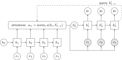
A recurrent network with an attention model: for each output the attention block compares the decoder state with all the of the encoder and outputs the context vector .
What radically new has happened here, and what else would we like to get rid of? First, in fact one can get rid of the input recurrent network entirely and keep only the attention model. That is the next step that was taken, and we will talk about it now: one can simplify this construction, get rid of recurrence, and this will also allow the process to be parallelised well. The second point is a generalisation: one can build trainable parameters into the similarity function and into the context vector . Note: in the attention model there are so far no trainable parameters to speak of; they are all contained in the functions , and . The idea is to introduce into the similarity function too matrices of weights that can be trained, and make a deeper network that enriches the attention model with additional parameters.
Applied problems
But first let us digress a little and think about where such models can be used. In fact their applications are far from limited to machine translation, although that is the first application on whose example this model was worked out.
Example (Applications of the attention model). Transforming one sequence into another, seq2seq:
- machine translation;
- question answering;
- text summarization;
- describing images, audio, video (multimedia description);
- speech recognition;
- speech synthesis.
For example, dialogue intelligence, the so-called chatbots, generating answers to questions: the input sequence is a question asked in natural language, the output a detailed answer, and the training sample must consist of questions and answers. The problem of text summarisation: a very long text is fed to the input, and one has to make a digest of it, keeping only part of the information at the output, but the most important part. Annotating images, audio, video: you have one sequence, for example a video, and you need to generate a running caption. Turning speech into text, speech recognition; speech synthesis. These are all examples of problems where it is very important, first, that you process the input sequence in small portions, that is, you can look ahead a little, and second, that in all these problems there is the notion of context. It is very good that the attention model allows us to formalise this context. And in all these problems the samples are large, and there is a need for parallelisation.
Interpretability: the attention matrix
What else is good about such models? Let us look at the example of machine translation. They allow one to figure out how it all actually works, and to make a visualisation like this.
Remark (The interpretability of the attention model). When a particular sequence is processed, visualising the matrix shows which words the model pays attention to when generating the word of the translation .
Attention matrices in machine translation from English into French (slide): a light cell is the word of the original that the model looks at when generating a word of the translation.
The matrix is of size "input length by output length" for the particular sentence we have just translated, and it is very easy to visualise. It turns out that the matrices perform a viewing of the context of each word in translation quite clearly and understandably for translators. Here the English phrase goes horizontally and the French one vertically. To translate the phrase "European Economic Area", we look at "zone économique européenne", in French the words go in reverse order, and so this thing arises here. The main thing is that the model discovered this thing, managed to determine the context correctly. Such a visualisation helps very well to understand in general how the attention model works, and to check purely visually whether everything is all right with it.
The attention model in generating image captions (slide): highlighted is the area the model looks at when generating the underlined word. K. Xu et al. Show, attend and tell: neural image caption generation with visual attention. 2016.
There are attention models for images too. How they are arranged we will not consider now; in a similar way, except that instead of a sequence there is an image at the input, and instead of a recurrent network there must be a convolutional one, and attention singles out certain areas of the image. The highlighted zone shows what we look at in the image when we generate a certain word of a natural language phrase; each word is generated in turn. For example, when we generate the word "stop", the attention model looks precisely at the "stop" sign. This allows one to understand that everything is happening sensibly: we really are looking at exactly what we are talking about now. A huge number of such works have been done; it is a very popular problem, in which there is substantial progress and fairly good quality of automatic generation of captions for pictures.
Varieties of attention models
Similarity functions and the "query–key–value" model
We have realised that there are several directions of generalisation, and first of all we want to introduce trainable parameters into the similarity function. What similarity functions are there at all?
Definition (Varieties of vector similarity functions).
- , the scalar product;
- , then turns into SoftMax;
- , with a matrix of trainable parameters ;
- , additive attention with .
Linear transformations of the query, key, value vectors:
, , are the weight matrices of linear neurons (trainable linear transformations into a space of dimension ).
A simplification of the model is possible: .
Dichao Hu. An introductory survey on attention mechanisms in NLP problems. 2018.
The first thing that comes to mind is simply to compute the scalar product. Fine; one can also transform it by the exponential, and then the normalisation operator turns simply into SoftMax. One can introduce a matrix of trainable parameters, and we get a bilinear form. One can do it differently: this is called additive attention, and we see that here a two-layer neural network is already built in as the computer of the similarity function; it has matrices and a parameter vector , that is, many trainable parameters have already appeared.
But the approach used most often is called query–key–value. Three types of vectors that figure in the attention model are introduced, and for each type its own linear transformation, which makes from the original vector a vector in some other space; all three are usually brought to one and the same dimension . The similarity function is the scalar product, but before taking it, each of the two vectors is translated by a linear transformation into a new space; in this way we give the model the possibility of training parameters, weight matrices. The query is the hidden state vector for which we want to generate an output: the word we want to generate in the output sequence acts as the query. That is, the query is a vector from the output sequence, but to compute the similarity function we transform it into a new space by the matrix . The key is the hidden state vector of an element of the input sequence: for each element the key is the vector , and we transform it too, but by a different transformation, . These two transformed vectors form the scalar product.
We divide by the root of , of the dimension. What is this coefficient needed for? It goes under the exponential in SoftMax and allows SoftMax to be made smoother. The trouble may be that as a result of the scalar product values that are too large or too small arise, too great a spread, and when the exponential acts on them, we will get a vector that tends to run off to zeros and a one. To prevent this, we divide by the root of the dimension. Why by the root? The scalar product of two vectors in a space of dimension is a sum of components; when we add many identically distributed random variables, the variance of the sum grows in proportion to , and the standard deviation as . Dividing by , we damp this growth of proximity values with the growth of dimension, and when we apply SoftMax to them, we get really good discrete distributions, not degenerate ones in which one probability tends to one and the rest are close to zero.
And one more generalisation: when we compute the context vector, we add up not the input vectors themselves but transformed ones; they are called value vectors. So we have three places where vectors are used, query, key, value, and in each of them its own transformation of the vector into a space of dimension is performed. The weight matrices of these transformations, read: of linear neurons in terms of a neural network, are what has to be trained. Sometimes things are simplified a little and the transformations of the key and the value are considered one and the same; in this way the number of parameters can be reduced.
The "query–key–value" attention model (slide).
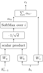
The "query–key–value" attention model: the query is compared by the scalar product with the keys , the result is divided by and normalised by SoftMax; the context vector is the weighted sum of the values .
The attention formula and self-attention
Let us generalise this and learn to write the attention model in a short form; I call it the attention formula.
Definition (The attention formula). is the query vector for which we want to compute the context; are the key vectors compared with the query; are the value vectors forming the context; is the estimate of the relevance (similarity) of the key to the query ; is the sought context vector relevant to the query.
The attention model is a 3-layer network computing a convex combination of the values relevant to the query :
is the example from the previous slide, where are the input vectors and the output one.
Internal attention, or "self-attention":
The terminology is this. There are vectors of three types: the query vector, for which we want to compute the context; the key vectors, which we compare with the query, in our example these are the elements of the input sequence, their hidden states, which we compare with the query to compute the proximity functions; and the value vectors, which we add up with these proximity coefficients, and in the end they form the context. Plus some relevance estimates for comparing the key and the query, how well the key suits the query; they can be computed in different ways. And the sought context vector, which is computed by this formula; we call it the attention formula, or the attention model.
What is it in essence? It is a three-layer neural network that computes a convex combination of the values relevant to the query. To remember and understand what an attention model is, one can try to make sense of this formulation. In fact everything here is very simple: one has to take and add up all the values, but with coefficients that show how important each of the values is for the given query. The values are the vectors we add up; the query in machine translation is the word we are generating, but not at all necessarily: in other problems it may be different, and we will now see an example of how differently one can treat what a query is. The keys and values are, as it were, tied to the input sequence, and the query to what we are trying to generate at the output.
The example from the previous slide is written briefly in one line through the function with three arguments, query, key and value, but now in vector form, so that it is visible how the weight matrices play here. Note that is already the matrix of all the input vectors, of size "dimension of the input vector by their number in the input sequence"; that is, the attention model can be written in matrix-vector form.
And one very important case that we will need later and with which we will mainly work is the internal attention model, or self-attention. This is when the input and output sequences are one and the same: we have no prime, we generate nothing, but want to transform the input sequence somehow. In this case is an element of the input sequence, the matrix of all its elements, and the queries are the elements of the input sequence, while the keys and values are all the elements of this same input sequence.
Multi-head attention
Let us see what modifications this general formula has. The first thing useful here is multi-head attention. It is called differently: in the English-language literature, multi-head attention, multi-dimensional attention; the Russian for "many-headed" sounds too much like a fairy tale, so in Russian we call it "multidimensional".
Definition (Multi-head attention). The idea: different attention models are trained jointly to single out different aspects of the input information (for example, parts of speech, syntax, idioms):
Variants of aggregating the output vector:
- , averaging;
- , concatenation;
- , to return to the needed dimension.
Regularisation: so that the aspects of attention are as different as possible, the rows of the matrix , , are decorrelated () and sparsed ():
Zhouhan Lin, Y. Bengio et al. A structured self-attentive sentence embedding. 2017.
The idea is very simple, and it is easy to grasp even on machine translation: translating a word, we pay attention to some other words, but with several attentions at once. To some words we pay attention by meaning, to some by grammar, by word forms; other words we may look at more attentively in order to swap them round or transform them a little, and so on. Some attention may be directed at finding out parts of speech, some at syntactic connections, some at idioms. That is, we need several attentions at once, and such a generalisation is very easy to write down: we introduce as many triples of matrices as needed and generate as many context vectors as needed; we decide ourselves, how many attentions we need in the model. When we immerse all this in a single huge deep neural network that will train all its parameters at once, these different attentions will automatically be tuned differently in order to achieve the result together. It is such a composition of attentions.
The question arises: how to aggregate these vectors into one big vector that we will use further? There are several strategies. The first is to average. The second is to concatenate, but with concatenation the dimension of the vector grows times. The third is to concatenate and then return to any needed given dimension with a linear transformation, which is also trainable.
One more point: here regularisation is often done, forcing all the aspects of attention to be substantially different. This trick was invented in the paper I give a reference to; it turned out to be fairly fruitful and is used in various subsequent works. The idea is to act on the matrix of coefficients so that the different attentions are different. We need to decorrelate the rows of this matrix so that the rows are as different as possible. How is this done? Recall that the rows are non-negative and normalised. So if we make their scalar products tend to zero, that will be a tendency towards orthogonality, the same as a tendency towards difference for non-negative vectors. And at the same time one can sparse: if the scalar product of a row with itself, that is, the squared norm of the vector , tends to one, it means that in the attention model we strive to concentrate attention on only one element of the input sequence. For machine translation this is exactly so: if you look at the attention matrices once more, you will see that for each element of the output sequence, generally speaking, only one element of the input one burns brightest. One cannot say that translation is literally word for word, but in most cases it is almost word for word, so we always look at some one word most attentively. The requirements of decorrelation and sparsing together give a very beautiful construction of regularisation: . Clearly, parameters sit inside the matrix , and when we include this regulariser in the overall quality criterion, we will of course have to run backpropagation through it too, and it will affect the optimisation of the parameter matrices of the keys and queries.
Hierarchical attention
One more construction is hierarchical attention.
Definition (Hierarchical attention). A nested structure: words sentences documents; are the words in the sentences .
The network of the first (lower) level, training sentence embeddings :
The network of the second (upper) level, training the document embedding :
Maximisation of the likelihood for classifying documents with labels :
Z. Yang, A. Smola et al. Hierarchical attention networks for document classification. 2016.
The idea is that when we do machine translation or in general do something with natural language, we work with texts that have a structure: documents divide into sentences, sentences into words. When, for example, we are doing not machine translation but want to classify documents, it means that, classifying a document, you must look attentively at certain of its sentences, those that contain the maximal information for classification, and in a particular sentence pay particular attention to certain words. That is, attention here is two-level, and let us formalise these considerations by means of the network architecture. The architecture is made two-level.
The lower level trains sentence embeddings: it works with words and at the output forms a sentence. The input elements are word embeddings, their vector representations, and the input sequence is processed by a recurrent neural network, a bidirectional GRU. I mentioned GRU a little when we had the lecture on recurrent neural networks; it is a kind of simplified LSTM. Bidirectional means that it forms hidden state vectors passing from left to right, then passes once more from right to left, and the two hidden state vectors obtained are simply concatenated. Then the vector goes for processing into a trainable transformation, which is simply one more layer of the neural network; in effect it forms the keys. Then the attention model works, and what is interesting here is that the query is simply some fixed vector, and a trainable one: one embedding for all sentences, which should show what one should pay attention to at all in order to classify documents correctly. Once more: we are now talking not about the machine translation problem but about the document classification problem, so there is no output sequence that we generate, and a fixed vector is used as the query. We simply need to learn to pay attention correctly to certain words and certain sentences in order to classify documents correctly. The query here is formed quite differently from the machine translation problem: there it runs over the words of the output sequence, while here it is simply a fixed vector, and it is unclear which one, so we must train it: is a trainable parameter of the model.
The network of the second level is arranged similarly. The difference is that the network of the first level gets words at the input and generates sentence embeddings , while the second level takes these sentence embeddings at the input and works with an input sequence that is in fact a sequence of sentences; about each sentence we have already figured things out at the first level. Then again trainable keys and again an attention model with a fixed query vector, but now . One vector, , says what to pay attention to in words; the second, , what to pay attention to in sentences. We do not know what exactly the attention model will learn at the lower and upper levels: it will depend on what the training sample is and by what features we want to classify the documents. Such a model of document classification, based on two-level hierarchical attention, turns out to be very good, competitive: it is able to solve text classification problems better than non-neural models, SVM and so on.
How do we train all this? Very simply: in the end a probabilistic model of document classification has to be formed. are the classes, for example the categories in a document categorisation problem; there may be very many classes. What is the logarithm of SoftMax over ? It means that there is a linear layer of neurons that takes as input the document embeddings formed by the model, and then a linear multiclass classifier works. This construction is nothing other than the loss function for a linear multiclass classifier whose document feature vector has been formed by a two-level attention model. A very useful structure for document categorisation problems.
The graph attention model GAT
One more thing I would like to tell before we talk about transformers is one more very important generalisation that is used more and more often in the most diverse applications: the attention model on graphs. We have already talked about graph embeddings, and the logic there was this: first we talked about texts, about how word2vec is arranged; there the notion of context appears, and we in effect build the vector representation of a word from all the contexts in which it appears. In graphs there is also, very naturally, the notion of a neighbourhood: if we consider a vertex of a graph and want to synthesise a vector representation for it, we must look at the vertices connected with it. In this sense a text is simply a special case of a graph, where each word is connected with the words that often go next to it in the same contexts. So everything invented on texts generalises easily to graphs through the notion of context, or neighbourhood.
Definition (The Graph Attention Network (GAT) model). The problem of classifying the vertices of a graph into classes .
Training data: , , ; are the input feature vectors of the vertices ; are the output vectors of estimates of the vertices, ; is the set of neighbours of the vertex , its context.
Multi-head self-attention, , on the vertex :
Maximisation of the likelihood (log-loss) over all parameters for multi-label classification of the vertices of the graph:
P. Veličković et al. Graph Attention Networks. ICLR-2018.
Let a graph be given and the problem be to classify the vertices of the graph over a set of classes . As training data, binary indicators that a vertex belongs to the class are used. Our main tool is the input feature vectors of the vertices and the output vectors of estimates of the vertices; the output vector is in effect the hidden state vector of a vertex, and let us build such vectors so that they predict the probabilities of classes: , transformed by the sigmoid activation function, should give an estimate of the probability of the class for the vertex . Our problem is in fact not only multi-class but also multi-label: each vertex of the graph may be assigned to several classes at once. So the probabilistic model is built not through SoftMax but through the sigmoid function for each class: for each class its own probabilistic model of the probability with which the vertex belongs to this class, and the sum over need not equal one.
Then everything is simple: we generalise the attention construction we had for texts to graphs. The difference is that we define the context for each vertex as the set of neighbouring vertices, directly connected with it by edges of the graph. In fact nobody forbids considering a neighbourhood of the second, third order, but for simplicity it is simply the set of neighbours. In general the whole construction can be defined independently of how you build this set of neighbours: it may be the result of a random walk, God knows what else; in each problem it can be defined in its own way. And now, the multi-head self-attention model. We already know what multi-head means and what self-attention is, when we look at one and the same sequence; here, besides the vertices of the graph, there is no other sequence, so it is self-attention. The vector we form for the vertex : it is the output vector of estimates; through the sigmoid it must give estimates of the vertex's membership in the classes, that is, in effect it is a description of the vertex that contains exhaustive information for classification over all classes. We sum over all the vertices that are nearest neighbours of . The query here is the vector of the vertex we are now classifying, the keys are the vectors of all the vertices from the neighbourhood, the values are again all the vertices from the neighbourhood. This is an attention model based on "query–key–value", and here the particular definition of the similarity function is through LeakyReLU, although another one could have been used.
How is the attention model on a graph tuned? The maximum likelihood criterion for our multi-label classification problem is simply written out. The vector representations have dimension , as many as there are classes, and through the sigmoid give the posterior probabilities of the classes for each vertex: a binary classification model for each class separately from all the others. As soon as the loss function has been written out, we understand that the whole set of model parameters figures here through the sigmoid and sits inside the attention model, the matrices and the vectors , , and we train them, naturally, by backpropagation, as usual.
GAT in the problem of classifying scientific papers (slide): the vectors projected by t-SNE; the colour of a point is one of 7 classes, the lines are the attention coefficients .
Example (GAT solves problems of classifying the vertices of a graph). The Cora, Citeseer, Pubmed datasets for classifying scientific papers by words (the features ) and the citation graph (the edges ).
What are such attention models on graphs used for? An example from the same paper: there are four datasets there, three of them problems of classifying scientific papers by their texts and the citation graph. There is information of two types: first, we see all the words in the documents; second, the links between documents, that is, which paper cited which. The words form the original features, and the graph is used to form neighbourhoods and apply the attention model. To illustrate that everything works sensibly, the authors show a projection by t-SNE; you already know that it is a way of multidimensional scaling. The problem was for seven classes, and the vertices of the graph really did split well into seven coloured parts. In places there are overlaps, but on the whole it means that quite adequate vectors were built for the vertices, and on them the classification problem into seven categories can be solved quite well. The paper shows that this works much better than the state of the art of other methods.
Transformers
The transformer for machine translation
Now we have the most interesting thing left for today: transformer models, neural network architectures based on the attention model, which are used first of all in machine translation. Again we refer to the paper "Attention is all you need", which is cited most often: in it the self-attention model was applied to make the best machine translation in the world.
We have considered several scattered stories not very connected with each other: attention models on graphs, hierarchical attention and multi-head attention. In transformers we will use multi-head attention and the attention formula; hierarchical attention and graphs we will not need now. If you missed something in those two pieces, no matter; the main thing is to understand what the attention model, self-attention and multi-head attention are.
Definition (The transformer for machine translation). The transformer is a neural network architecture based on the attention model and fully connected layers, without RNN.
The scheme of data transformation in machine translation:
- , the words of a sentence in the input language; ↓ trainable or pre-trained vectorisation of words
- , the embeddings of the words of the input sentence; ↓ the transformer encoder
- , contextual embeddings of the words; ↓ the transformer decoder, similar to the encoder
- , the embeddings of the words of the output sentence; ↓ generation of words from the language model built
- , the words of the sentence in the output language.
A. Vaswani et al. Attention is all you need. 2017.
By what scheme is machine translation done? There are the words of the original sentence in the input language. Clearly, we consider words as vector representations, embeddings, and there are two options here: either the embeddings are trained by the model itself, that is, they are its parameters, its own embedding for each word, one and the same globally over the whole collection, or they are pre-trained: there is some other model, for example word2vec, that has already built word embeddings, and we use them as input data, while the model does not train them. Both options are used, depending on how big your data are: if the data are gigantic, they allow the embeddings of all words to be trained.
So, first, the original words are translated into embeddings. Then the transformer works. Briefly, a transformer is self-attention models placed one after another, which translate the original sequence of vectors into new vectors that encode information about the context of each word very well and correctly. The transformer encoder translates the vectors of the original words into certain hidden vectors that correctly preserve in themselves information about the context of each word: represents the word itself and does not yet know anything about which words it stands next to in the sequence, while contains information about the context of the word . is what we have encoded the input sequence into, the result of the encoder. We need one more transformer that will carry out decoding: to transform the original sequence of length into the output one of, generally speaking, a different length, which will consist of embeddings of words of the output language. And the last element is to generate the words themselves from these embeddings; here a probabilistic language model works, and we will also see how it is arranged. That is, the machine translation scheme consists of four transformations: words into vectors, word vectors into context vectors, context vectors into vectors of the output language, and then from these vectors, words. This is the general pipeline of machine translation, and clearly it is also an encoder–decoder.
The architecture of the transformer encoder
Let us consider the encoder more carefully. There are very many auxiliary subtleties here, so I have taken the picture from the paper and marked on it step by step what vectors we get. This slide is a compilation from a large number of different papers, popular and less so: nowhere did I see the whole structure of the neural network with all its parameters shown just step by step; I had to figure this out. For understanding transformers this slide is absolutely key.
Definition (The architecture of the transformer encoder).
- Positional vectors are added:
- Multi-head self-attention:
- Concatenation:
- A skip connection + layer normalisation:
- A fully connected 2-layer network FFN:
- A skip connection + layer normalisation:
The transformer encoder (slide): the picture from the paper with the vectors of steps 1–6 marked.
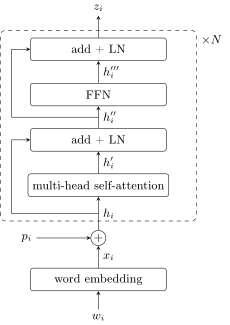
A block of the transformer encoder (steps 2–6, in the frame, are repeated times): multi-head self-attention and a two-layer FFN network, each with a skip connection and layer normalisation LN.
Let us go step by step, from top to bottom. The input words first enter the embedding block; we will not consider it in detail; the main thing is that we have got a vector representing the -th word. What happens to this vector? First of all we need somehow to remember information about the position of this word in the input sentence: originally the embedding of the word does not have this information; it is simply a vector representation of the word, which knows nothing about what sentence it is used in. So so-called positional vectors are added to . They can be built in different ways, we will consider that separately below, but now remember one simple thing: an addition is added to the original vector representations of the words, with the property that the farther apart two words are in the sentence, the greater the distance between their additions. The function of this addition is to make the embeddings of words more distant from each other if these words are far from each other in the sentence.
Next the formed vector is fed to the input of multi-head self-attention with trainable matrices for the query, key and value. I write out in small print what dimensions figure here: in this 2017 work all hidden state vectors had dimension 512, and there were 8 attention heads. And the authors came up with a very elegant trick: let the three transformations translate the original vectors of dimension 512 into vectors of exactly 8 times smaller dimension, 64. It turns out that we build 8 attention models, each working in a space of smaller dimension 64, and then, when we concatenate 8 times 64, we return to the original dimension 512.
Next the authors say that the vectors at the output of multi-head self-attention require one more additional trainable transformation, and they add a fully connected two-layer neural network that transforms these vectors through two layers. But before subjecting them to this transformation, two more very important transformations are done with them. First, they are normalised: at the output of eight attention models one can get vectors measured on slightly different scales, so a so-called normalisation has to be done, layer normalisation; it has two trainable parameters for each dimension of the vector; below I will show in detail how it is arranged. Second, the skip connection. Remember residual networks? We have already mentioned this once or twice: when ResNet appeared in the ImageNet competition, another sharp leap happened. Skip connections are arranged very simply: the input vector is simply added to the output one. Normalisation and the skip connection are the "Add & Norm" block, the two-layer network is "Feed Forward". It is interesting that in this two-layer network the intermediate hidden layer was for some reason made very large: this is not an encoder that reduces the intermediate dimension of the representation but, on the contrary, it increases it (2048 against 512). This adds degrees of freedom and allows the vector to be transformed into so that this transformation is quite non-trivial, transforms the original representation in some complex nonlinear way to get new vectors, more informative, more aimed at forming the correct context vectors. And the last thing is once more layer normalisation and a skip connection: steps 4 and 6 are analogous to each other.
That is the transformer encoder. Yes, I forgot to say: steps 2–6 form one block, and 6 such blocks are stacked on top of each other. Not only did we make the self-attention model multi-head, not only did we transform its output by a two-layer fully connected network, but from this we formed one transformer block, which transforms the vector representations of words into new vector representations of contexts, makes from . And we apply six such transformations one after another: six times we make contexts from contexts. In this way we enrich the model, increase the number of parameters, and clearly such a model has to be tuned on some super-huge collections of text documents.
Remark (A few additions and remarks).
- The computations are parallel over the elements of the sequence , which would be impossible in an RNN.
- blocks are connected in sequence.
- Pre-trained embeddings may be used.
- Embeddings of the words may be trained: , or in matrix notation , where is the vocabulary of the words of the input sequences, the matrix of trainable vector representations of words, the matrix of binary (one-hot) encoding.
- Layer Normalization, :
A few additions and remarks. First, what is remarkable about the attention model at all: the computations here can be parallelised, which would be impossible in an ordinary recurrent network. That there are 6 such blocks one after another I have already said. Why 6? In fact it is simply the choice of the authors of the paper; in subsequent models both 12 and 24 were used; it is a parameter that can be increased to extend the descriptive abilities of the model. Where do the embeddings come from? Different options are possible: one can use pre-trained ones, or one can train them. How? One can do so-called one-hot encoding: each word must have its own embedding. In matrix form this is written like this: you have a vocabulary of the words of the input sequences and a matrix of trainable vector representations of words of dimension by the size of the vocabulary. Each word is originally encoded by a vector of dimension equal to the size of the vocabulary, in which there is one one, and only in one place. Clearly, you will most likely not form and store such highly sparse vectors explicitly; the point is that for each word its own trainable vector is formed, and it is these that are the parameters of the network. This matrix you really do train.
And the last remark: how layer normalisation is arranged. You take the input vector of dimension ; it is the vector that arose after the attention model, after you concatenated all the heads, all 8 attention models, and got the vector representation . The trouble with this vector representation is that one attention model may have got one distribution of values at its output, and another a quite different one; this has to be evened out somehow. You compute the mean and the variance over the whole vector , for the stability of the normalisation; they are not trainable but simply computed from the vector itself. The vector is centred and normalised, and then each coordinate is transformed by its own trainable linear transformation with two parameters, and . From the formula it is seen that this is simply a linear transformation, and in a neural network architecture it is very easily implemented, simply one more layer of the neural network. And, as you see, in this layer a skip connection is also added: to the input vector you add what came to the input of the previous layer, that is, to the input of the attention model.
Positional encoding
And the last remark about the transformer encoder: positional encoding.
Definition (Positional encoding). The positions of words are encoded by vectors , , so that the greater , the greater , and is not bounded:
A more modern way of taking relative positions into account:
where is the truncated difference, .
A. Vaswani et al. Attention is all you need. 2017. P. Shaw, J. Uszkoreit, A. Vaswani. Self-attention with relative position representations. 2018.
The point is very simple: the position of a word, the number of the place in the input sentence where this word stands, you must transform into some vector of the same dimension so that two requirements are met. First: the farther apart the positions and , the greater must be the distance between the vectors. Second: we do not know the length of the input sequence, it may be anything at all, that is, the encoding mechanism has to be devised so that this property remains valid regardless of the length of the sequence. This can be done in different ways, and in the original paper this sine-cosine transformation was proposed. In the picture it is well seen: is the number of the position, we consider a sentence 20 words long, and we understand that with sines and cosines the generation can be continued further down: whatever the length of the sentence, 50, 100, 500, we will continue generating these waves. And the property really is such that the farther apart two rows are, the greater the distance between them.
The positional vectors for , (slide): the left half is sines, the right half cosines.
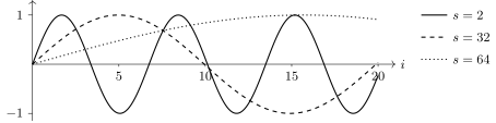
The coordinates of the positional vector as functions of the position with : as the number of the coordinate grows, the frequency falls, and together the coordinates distinguish positions at all scales.
Of course the question arises: why sine and cosine? Some complete arbitrariness, and moreover we literally add these vectors to the vector representations of the words; it seems a rather strange model. In fact a better and more modern way was invented a year later, partly by the same authors. They proposed moving away from sines and cosines and using simply an attention model to take relative positions into account. It is arranged as follows: a trainable correction is added to the keys and values, and there are comparatively few parameters in it. It depends on the difference , a truncated one, a kind of local difference: if two words and are more than apart, the difference simply equals , and if less, it is simply the difference . The corrections are indexed by values from to , that is, there are only of them; is the size of the neighbourhood for which you want to introduce positional corrections. If a pair of words is located more than apart, the same positional correction goes for it as for . And an attention model is introduced that allows the original sequence to be re-encoded into a slightly corrected one, by way of, by and large, insignificant further training.
The architecture of the transformer decoder
That is all about the transformer encoder. Now we are armed with all the knowledge to understand how the decoder works, and there is nothing terrible there: everything is repeated in the image and likeness.
Definition (The architecture of the transformer decoder). Autoregressive synthesis of a sequence: is the embedding of the start symbol; for all :
- Masking the "data from the future":
- Multi-head self-attention:
- Multi-head attention on the encoding :
- A two-layer fully connected network:
- A linear predicting layer:
generation , while .
A. Vaswani et al. Attention is all you need. 2017.
The transformer encoder and the transformer decoder (slide): the output of the last block of the encoder is fed into the middle attention of each block of the decoder.
Again the picture from the paper, but here I show a few more labels. In the large blocks I write: multi-head self-attention plus layer normalisation; you should already understand that this is a superposition; it corresponds to the orange square, which does multi-head attention, and the yellow one, in the image and likeness, exactly the same block as in the transformer encoder. Let us consider what is specific, how the decoder differs from the encoder.
The main thing is that the output of the encoder must somehow get into its input, and it gets in here, into the middle. In grey the decoder block is highlighted, and it differs from the encoder block in that one more multi-head attention has been inserted into it. The first is self-attention, and the second is not self-attention but attention to the vectors obtained from the last block of the encoder. In the encoder there are six blocks on top of each other, and at the output of the last block the final vector has formed, the hidden representations of the contexts of all words. They are fed to the input of the decoder blocks, of which there are also 6, and each block is fed the output of the sixth block of the encoder. That is, the blocks are not connected with each other in pairs: only the last block of the encoder gives information to all the blocks of the decoder.
Let us figure out the finer details. The decoder should be similar to a recurrent neural network, but one wants to move away from recurrence and make it so that the decoder too can be parallelised, while the words are generated one after another. How are these seemingly incompatible things to be combined? A very simple trick helps here, which is called masking: you forbid yourself to peek at the words you have not yet generated. The key point is that is the matrix of hidden representations of words that encodes the output sequence, but only up to the -th position. The final length of the sentence at the output will be , but, generating the -th word, you are entitled to look only at the previous ones, up to the previous one.
So, first you do, naturally, the positional embedding and agree that at the input of the subsequent layers you will use only the vectors of the words you have already generated. Next comes multi-head self-attention; it is called masked multi-head attention precisely because the keys and values are applied not to all vectors but only to the vectors you have already synthesised in the output sequence. All this is still synthesised one after another, but the synthesis of each relies only on the previously synthesised ones. Next, multi-head attention on the encoding you got from the encoder; this is not self-attention but ordinary attention, because the transformed vectors are used as the keys and values. In architecture this is an already familiar construction: layer normalization and multi-head attention. After the self-attention block you have analysed the sequence you have already generated by this moment; after the attention block you have looked at the context in the input sequence; after that you once more do a two-layer fully connected feed forward network, by analogy with the encoder, and at this moment you get , the vector with which you predict the word.
And the last, fifth level is executed after you have executed the decoder blocks six times one after another, applied attention models very many times, with their own trainable parameters in each block. "Linear + SoftMax" is in effect a linear predictive model with SoftMax, which is the language model: for each position of the output sequence a probabilistic model of the language is built, that is, all the words from the output vocabulary get probability values, and they are obtained from the vectors taken from the last block of the transformer decoder. This is an ordinary one-layer neural network: is a trainable matrix of weights, an offset vector, also trainable, which gives the probabilities of the classes at the output, and the classes are all the words. That is, for each word position you solve a multiclass classification problem in order to understand which word is best put in this position. And then you generate the words themselves. How, having a probabilistic generative model for words, to actually generate words is a separate topic, with many subtleties there; for simplicity one can consider that for each position the most probable word is simply chosen. This is done until you generate the word denoting the end of the sequence. There is also begin of sentence, the embedding of the start symbol: generation has to start from something, at there must be some , and it too is a trainable vector, the embedding of the start symbol. And in exactly the same way there is an end symbol: when you see that the most probable token at the output is the end symbol, it means you have generated the sentence completely.
Clearly this is a very complex encoder and decoder, two transformers. What is a transformer? Attention blocks placed in sequence, each of which transforms the vector representations of all the elements of the input sequence.
Criteria for training and evaluating machine translation
The last thing left to understand is how all this is trained, by what criteria.
Definition (Training and validation criteria for machine translation). The criterion for training the parameters of the neural network on a training sample of sentences with the translation :
Criteria for evaluating models (non-differentiable) on a sample of pairs of sentences "translation , reference ".
BiLingual Evaluation Understudy:
Word Error Rate:
A. Vaswani et al. Attention is all you need. 2017.
The machine translation problem. Let us denote the totality of all the parameters of this most complex neural network by . There is a training sample in which there is an original sentence in the input language and its translation into the output language. The criterion for training is a sum over all pairs of sentences, then a sum over all the words of the output sentence, and a probabilistic language model is trained that at the last step gives conditional probabilities for all words: each word of position of the output sequence figures in this probabilistic language model under the logarithm. This is the principle of maximum likelihood: how well the model describes the appearance of the words we see at the output. Clearly this is a good differentiable criterion, so that backpropagation works and we can train this whole very multilayer construction. Here there really is a very deep neural network. Reckon it up: the attention model is three layers, plus normalisation, one more, plus a two-layer network with normalisation, three more, that is, 7 layers just in each encoder block, and there are six of these blocks. In the decoder it is 4 plus 4 plus 3, that is already 11, and there are also 6 such blocks. An impressive depth results, and you train this whole deep network by this criterion with backpropagation.
Machine translation, however, is customarily evaluated by somewhat different criteria. I give the formula, but would not like to dwell on it. The BLEU metric (bilingual evaluation understudy) was invented long ago for machine translation: it shows how well a phrase generated by an algorithm corresponds to the reference phrase. We simply look at how many coinciding words there are, coinciding bigrams, trigrams and 4-grams; usually one stops at four. An additional penalty is also introduced for our regularly making shortened translations: if the total length is regularly less than needed, it means that the model for some reason spits out the end-of-sequence sign earlier, and this has to be corrected; we penalise for it. Sometimes an even simpler quality criterion is used, WER, which simply measures the number of insertions, deletions and substitutions in each sentence compared with its correct version, the reference.
The transformer encoder BERT
The BERT model
What more good can be said about transformers? The BERT model is an already very well-known model for language processing, in effect "our everything" since 2019: in the last two years everything done in neural networks for natural language is in one way or another similar to BERT or is its further development or modification; at least, these too are some transformers. Transformers are the state of the art for text processing.
Definition (BERT (Bidirectional Encoder Representations from Transformers)). The BERT transformer is an encoder without a decoder, pre-trained on a large text collection to solve a wide class of problems of automatic text processing.
The scheme of data transformation in NLP problems:
- , the tokens of a sentence of the input text; ↓ training embeddings together with the transformer
- , the embeddings of the tokens of the input sentence; ↓ the transformer encoder
- , the transformed embeddings; ↓ fine-tuning for a particular task
- , output text / markup / classification, etc.
J. Devlin, M.-W. Chang, K. Lee, K. Toutanova. BERT: pre-training of deep bidirectional transformers for language understanding. 2019.
The BERT model, unlike the machine translation model, takes only the encoder: at the input for training simply a body of texts of some language is given, and that is all. So the question arises by what criterion to tune it; we will certainly come back to this. Compared with the previous model, this variant is simpler: there were four steps there, and here three: the tokens, the words, are translated first into embeddings, then the transformer encoder works and forms the context embeddings , and then we use them to predict something. And very different things can be predicted, and the whole beauty of the BERT transformer lies in the fact that the first two transformations can be trained jointly on a very large collection of texts, unlabelled ones at that: there is neither translation nor classification for them, no markup, it is just text. The only thing in these texts is information about how words follow one another, how they appear in the contexts of their sentences, and this is exactly what gives the idea for the criterion for training the transformer. BERT is such a universal encoder: it is pre-trained once on a very large collection, and then the first two transformations can be used to solve other problems, and the model fine-tuned on perhaps not very large samples for specialised tasks.
Criteria for training BERT: MLM and NSP
How does training happen? There are two criteria.
Definition (The MLM criterion (masked language modeling) for training BERT). The masked language modelling criterion MLM is built automatically from texts (self-supervised learning):
where is a subset (15 %) of masked tokens from ;
is the language model predicting the -th token of the sentence ; is the contextual embedding of the -th token of the sentence at the output of the transformer encoder with parameters ; are all the parameters of the language model.
The first criterion is masked language modeling. It is a very simple thing: you, as it were, cover, mask 15 per cent of the words in sentences and say: I want to teach the model to predict these words from the context. That is, looking at a sentence and having covered 15 per cent of the words in it, you want to predict these words correctly. The masking model is also a language model: you predict the probability of words for each word position. Here is precisely the output of the transformer encoder, that is, all the main parameters sit in this model; at the output for each word position you get some vector and use a one-layer linear classifier to synthesise words from these vectors, build such a language model and train it by the maximum likelihood principle. You train the transformer model to predict the covered words correctly; the sample indicates which words are masked.
Definition (The NSP criterion (next sentence prediction) for training BERT). The criterion of predicting the connection between sentences NSP is built automatically from texts (self-supervised learning):
where is the classification of a pair of sentences;
is the probabilistic model of binary classification of the pairs ; is the contextual embedding of the token for a pair of sentences written in the form .
The second criterion is to predict whether two sentences follow one another. A special training sample is formed, and it has the original text form: two special tokens are introduced, an initial token and a separator token, and two sentences and follow one another. The criterion is a sum over all pairs of sentences, and for some pairs it is known that they follow one another, and for some that they do not, and you are classifying pairs of sentences encoded in this text form. One has to solve a two-class classification problem: learn to recognise whether this is a pair of sentences that followed one another in the original text, or random sentences that have nothing to do with each other. You use the contextual embedding: the same transformer encoder is simply applied to such a sentence; it too is text, only specially composed of two sentences, and two tokens are specially embedded in it. In effect you make a prediction for the token of this pair: it can be asked whether these sentences follow one another or not. To build such a two-class classification model, you take the embedding BERT gave at the output and feed it to the input of a two-layer fully connected neural network; this model of classifying pairs of sentences is trained by the maximum likelihood principle.
These are the two criteria used to train BERT. They are trained jointly, on the two criteria with some weights, that is, simultaneously on one criterion and on the other.
Fine-tuning and model sizes
Remark (A few more remarks about transformers).
- Fine-tuning: for fine-tuning for a task, a model , a sample and a criterion are given.
- Sets of test tasks on language understanding (GLUE, SuperGLUE).
- Transformers are usually built not on words but on tokens obtained by BPE (Byte-Pair Encoding) or WordPiece.
- The first transformer: , , , 65M weights.
- , GPT-1: , , , 110M weights.
- : , , , 340M weights.
- GPT-3: 175 billion parameters.
A few more remarks about BERT and BERT-like algorithms, about how they are customarily used to solve other problems. BERT itself is trained on a huge, unthinkable collection of texts; the GPT models are trained in a similar way, they too have transformers, the training criteria differ slightly, but on the whole these are very similar models. When you face a particular task with its own loss function, you can do fine-tuning. You have a model of contextual hidden representations for sentences, what BERT gives at the output of the transformer, and on top of these vector representations you can solve your problem: classify sentences, some fragments in sentences or whole documents. Today we saw such examples: the hierarchical attention model was an example where a multi-class, multi-label document classification problem is solved; you can do something similar. Fine-tuning means that you switch on backpropagation through the whole of BERT and train not only the parameters you need but also further train the parameters of BERT itself. One may also not do this: keep the model that was pre-trained on a large collection and train only the parameters of one's own task proper.
Next: there are remarkable test sets of tasks on natural language understanding. These really are challenges, very hard problems, and datasets have been formed from them through which different transformer-like models can be run at once. It is a kind of multi-task platform for testing pre-trained models, which need not repeat the BERT architecture, may be arranged very differently, differ in various nuances; testing on such multi-task datasets allows one to understand how well you are doing language modelling for language understanding, that is, for solving very many different tasks at once.
And one more piece of news with which I want to stun you: I never once said this; I kept saying that we encode the words of the input sequence, then word embeddings, but in fact everything is arranged a little more cunningly; I was simplifying. One can work on words too, but both BERT and the transformer for machine translation, generally speaking, work on the technique of byte pair encoding or WordPiece. What is that? Briefly: you cut words into pieces and then form a vocabulary of pieces or subsequences of these pieces that occur often in the collection. You get a vocabulary in which about half are real words and half some stubs of words. What is good about such encodings? They also allow the vocabulary to be reduced: for example, in languages like Russian, where there are very many word forms, it becomes possible to store word roots separately and parts such as endings, suffixes, prefixes. But this is done not explicitly but by an automatic procedure of forming a vocabulary in which both words and pieces of words stand on an equal footing.
Once more the parameters. The transformer for machine translation has 65 million weights. The base BERT model and the GPT-1 model are already weightier, one and a half to two times: 110 million parameters. The widest BERT already has 340 million parameters. And GPT-3 has 175 billion parameters, orders of magnitude more again.
Summary
Remark (Summary).
- Attention models were first built into RNNs, but later it turned out that they are self-sufficient.
- The attention model works more accurately and faster than RNN: the computations and the training parallelise better; the model is easily pre-trained and used for many tasks; it generalises successfully to graphs, images, video.
- It has been proved that the multi-head self-attention (MHSA) model is equivalent to a convolutional network [Cordonnier, 2020].
- The attention model underlies transformers and the large language models BERT, GPT-3 and others.
A. Vaswani et al. Attention is all you need. 2017. Dichao Hu. An introductory survey on attention mechanisms in NLP problems. 2018. Xipeng Qiu et al. Pre-trained models for natural language processing: a survey. 2020. J.-B. Cordonnier et al. On the relationship between self-attention and convolutional layers. 2020.
To sum up briefly. First: attention models are the key point, a building block for very many modern models, not only transformers but also models on graphs. The attention model is in fact very simple, and it is a kind of advanced model of context. Context models of the word2vec type are after all rather trivial: we simply predict whether words will stand somewhere side by side, often occur in the same contexts. The attention model is much deeper: it models which parts of sequences one has to look at when generating output sequences. And it is good that the attention model moved away from the recurrent neural network for the input sequence: we have completely got rid of the need to process words one after another and so can parallelise. The attention model parallelises very well, generalises very well to graphs, images and so on; very many different problems are already being solved with it.
Remark (A question: is the attention model not an advanced variant of a convolutional network). There was a question: it seems that the attention model is after all a kind of advanced variant of a convolutional neural network; is that so? There is a paper from last year, 2020, which really does show that the multi-head self-attention model is equivalent to such a specific convolutional network.
And the transformer is multi-head attention models interleaved with layers of fully connected neural networks, a very deep architecture. It is the base architecture for practically any advanced language models, BERT, GPT-3 and many others; dozens of them have appeared literally in the last three years. The topic is very rich; one could give a whole course on it, and it is hard to fit into one lecture.
No comments yet
Be the first to share your thoughts.