August 30, 2026 · Lecture · LibreTimes
Machine Learning 2. Lecture 3. Vector Representations of Texts and Graphs
Contents
- What this lecture is about
- Vector representations of text
- The distributional semantics hypothesis
- The CBOW model
- The Skip-gram model
- Comparing CBOW and Skip-gram
- Hierarchical SoftMax
- Skip-gram with negative sampling
- The connection of word2vec with matrix factorisations
- What word vectors are for and how they are checked
- The FastText model
- From texts to graphs
- Multidimensional scaling
- The multidimensional scaling problem
- Multidimensional scaling for data visualisation
- Stochastic neighbour embedding (SNE)
- Perplexity
- t-SNE
- Vector representations of graphs
- Matrix factorisations
- Random-walk models: DeepWalk and node2vec
- Graph autoencoders
- A reminder: autoencoders for semi-supervised learning
- Vector representations of graphs as autoencoders
- GraphEDM: a generalised autoencoder on graphs
- Graph neural networks
- Summary
- Seminar
What this lecture is about
Today's lecture continues the story of neural network models, and it has a substantial link with the previous one, where we looked at autoencoders and, in general, at vector representations of input objects with a complex structure. Today the whole lecture is, in essence, about exactly that. We will consider two types of complex structured objects: natural language texts and graphs. There will be many methods, and among them is t-SNE, a very interesting method for the visual representation of data, which, although it is known first of all as a visualisation method, can in fact be regarded as a way of embedding graphs.
We will begin with texts, and then we will see that texts are a special case of graphs, and move on to graphs.
Vector representations of text
The distributional semantics hypothesis
Let us begin with a seemingly purely linguistic thing, the distributional hypothesis. The word has nothing to do with the distributive law in arithmetic: it should be understood in the sense of distribution, literally a probability distribution. The question is how to define formally what the meaning of a word is. When linguists thought deeply about this, and they worked on it in the middle of the last century, the following understanding appeared: the meaning of a word can be defined as the totality of all possible contexts in which this word appears anywhere at all in the language, for example in all the sentences that have ever been written or spoken anywhere.
Definition (The distributional hypothesis). "The meaning of a word is determined by the set of its contexts".
- Words that occur in the same contexts tend to have similar meanings [Harris, 1954].
- You shall know a word by the company it keeps [Firth, 1957].
Z. Harris. Distributional structure. 1954. J. R. Firth. A synopsis of linguistic theory 1930–1955. Oxford, 1957. P. Turney, P. Pantel. From frequency to meaning: vector space models of semantics. 2010.
Clearly this definition is not constructive. If we translate the statements of the classic linguists: the meaning of a word is determined by all its contexts; words close in meaning appear in close contexts; a word is characterised by the company of words in which it appears. These principles make up the meaning of the distributional hypothesis: we would like to describe words somehow by their contexts, and the notion of context has to be formalised somehow.
There are two more interesting and closely related linguistic notions here: syntagmatic and paradigmatic similarity of words.
Definition (Syntagmatic and paradigmatic similarity of words). Syntagmatic similarity is the co-occurrence of words in one context (building — builder, tap — water, function — point).
Paradigmatic similarity is the interchangeability of words in one context (building — house, tap — faucet, function — mapping).
Syntagmatic similarity is the kind we observe explicitly in a text: words that appear in a common context go together with each other; they do not necessarily stand next to each other, perhaps a few words apart. "Building — builder", "tap — water", "function — point": these pairs of words very often go in the same contexts, appear side by side. Paradigmatic similarity, by contrast, is unobservable: it is about one word being replaceable by another. It is something like synonymy, but not quite; it is the interchangeability of words: "building — house", "tap — faucet", "function — mapping". You do not see that one word can be substituted for another in a given particular context, but somewhere else, in the terabytes of texts that exist somewhere, exactly the same context can be found, and in it another word will stand in place of the given one. That is paradigmatic similarity of words. It is conditionally observable: in principle you observe it somewhere, but just try finding that place in terabytes; that is a technical problem too. And this concept appeared back in the years when there were neither big text data, nor efficient search mechanisms, nor search engines, yet the notion of the distributional hypothesis had already arisen.
The CBOW model
Let us try to formalise this notion. How do we set ourselves the problem? We have a huge number of texts: the whole of Wikipedia, the whole Encyclopaedia Britannica, the whole internet, some terabyte of text; in short, natural language texts. We want to represent each word by a vector in a space of a given dimension so that words close in meaning have close vectors. This is where the distributional hypothesis comes to our aid: it allows us to formalise what "words close in meaning" means. If the linguists had not given us such a hint, we as engineers would be a little at a loss here: what is the meaning of a word? Fortunately, we are given such a formalisation.
Let us take this as far as mathematical formulations of the problem. There were two models here. The first is called continuous bag-of-words. In general, in text analysis a bag of words means a representation of a text in which the order of words does not matter: all the words in a text can be shuffled randomly, swapped around, and the analysis should not change because of that. There are many such methods; linguists naturally criticise them for not taking word order into account: how can that be, it matters in language. Nevertheless, continuous bag-of-words is a model that assumes that word order is not very important in the neighbourhood of a given particular word. A text as a long chain of words preserves order on the whole; order is not preserved only locally, in a small neighbourhood of each word. We consider a neighbourhood of radius : from the word we take words to the left and words to the right, a sliding window. We go along the text, and for each word we consider such a window.
Definition (The CBOW model (continuous bag-of-words)). Given: a text , a sequence of words of the vocabulary .
Find: vector representations of words such that words close in meaning have close vectors.
The model of the probability of the word in a given context :
where is the mean vector of the words of the context ; are the vectors of the predicting words; is the vector of the predicted word, in general .
Criterion of maximum log-likelihood, :
We build a probabilistic model: we want to predict the word in the -th position from its context, that is, to learn to build the conditional distribution . The parameters of this model will be the vector representations of words. What do we do? First, we form a vector representation of the context: we take and average the vector representations of all the words in the window of width ; the word itself is excluded, we do not take it into the context. Since it is a sum, we have already lost the word order: we have lost the information about the order of words within the context, and here it no longer interests us. Then we take the scalar product of the vector of the given word and the mean vector of the words of the context, and pass it through SoftMax over the whole vocabulary.
Note that is not the same as : here we introduce two alternative vector representations for each word. When a word is in the context, it is a predicting word, it is used to predict the word ; and when the word is itself predicted, another vector is taken for it. A question arises at once: can they be combined, can one and the same vector representation be used for these two roles? Generally speaking, yes, and such models exist too, and they also work quite well. But for generality, if we want to enrich the model, two different vector representations can be used.
It remains to take the last step. We have a probabilistic model of word generation, and it has parameters, the vectors and . Let us take our whole text collection as the training sample and apply the maximum likelihood principle: the sum of the logarithms of our probabilistic model over all word positions in our big text. The parameters are in essence two matrices of size "vocabulary size by the dimension of the word vectors", and these are what we will look for.
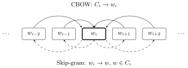
A sliding window of width around the word . CBOW predicts the word from the mean vector of its context (solid arrows), Skip-gram predicts each word of the context from the word (dashed).
The Skip-gram model
Next, naturally, a problem arises: how to solve such a problem, what pitfalls there are in terms of optimisation and how to get round them. But first, one more, alternative formulation of this problem, which is called skip-gram. N-grams are consecutive words, and in text analysis skip-grams is the usual name for n-grams from which the word of interest has been thrown out, dropped; hence "skip": some words in the n-grams are skipped. The problem is the same, the "given" and "find" are the same, but the model is different. Whereas in CBOW we predicted a word from its context, here we will do the opposite: predict the words of the context from the word .
Definition (The Skip-gram model). Given and find: as in the CBOW model.
The model of the probability of the words of the context given the word :
is the vector of the predicting word, the vector of the predicted word, in general .
Criterion of maximum log-likelihood, :
T. Mikolov et al. Efficient estimation of word representations in vector space. 2013.
What difference would it seem to make? The difference is that no averaging of vectors takes place here: we simply predict one word from another. The model is very similar, the same SoftMax, the construction slightly different: we go over all word positions, for each word position we go over all the words of its context and try to predict each word of the context from the word in position . The predictive model is the same, SoftMax of scalar products of word vectors, and here too the vectors of the predicting words and the vectors of the predicted words are distinguished. In principle it is possible to set them equal to each other, but usually they are still not set equal.
Comparing CBOW and Skip-gram
So as not to get confused, let us write these two models out side by side and see what the difference is.
Remark (Comparing the CBOW and Skip-gram models). The difference is in the structure of the optimisation criterion:
- Skip-gram models the probabilities of rare words more accurately.
- Both models can be trained by SGD.
- Both models are implemented in the word2vec program [Mikolov].
- Both criteria are hard to optimise because of SoftMax.
- What to do? Replace either SoftMax or the criterion.
The difference is, in fact, in where the sum over the words of the context stands in the criterion: in CBOW the sum is under the SoftMax, and in Skip-gram it is outside the SoftMax. That is the whole small formal difference between the two criteria that formalise the principle of distributional semantics.
What is known about which of the two models is better? It seems that Skip-gram is usually preferable: it is said to model the probabilities of rare words more accurately. Both models can be trained by stochastic gradient, and that is what is done; both are implemented in Tomáš Mikolov's program word2vec. But optimising either criterion head-on is very difficult. Why? SoftMax is an unpleasant function. Note: SoftMax turns a vector into a normalised vector, and the normalisation is over all the words of the vocabulary, that is, in the denominator of each SoftMax sits a sum whose number of terms equals the size of the vocabulary. This whole contraption has to be differentiated; this denominator will have to be computed, there is no getting away from it, and that is of course very bad computationally. So one has either to learn to compute SoftMax efficiently, or to replace the criterion altogether and use something simpler instead of SoftMax. These are exactly the two paths people took, and the existing efficient implementations in fact optimise a criterion slightly different from the one written out above. Let us figure out how this can happen.
Remark (A question: what is the point of the two models, and what is a context). The point of one model is to skip one word and predict it from the context; the point of the other is to predict from one word not the text, as it were, but a small neighbourhood of this word. The context can be defined in different ways. Often one simply takes words, where is of the order of five to ten, that is, a small number of words. One can take the sentence in which the given word is located; then the contexts will be of different lengths, different on the left and on the right, and everything will be more complicated. Generally speaking, both formulations can be regarded as a modification of a more general concept: we want to predict whether two given words occur next to each other. It seems that both models are doing exactly that, and a little later we will see that this is indeed so, despite the outward difference.
Hierarchical SoftMax
So how is the problem with SoftMax, which causes us so much pain, solved? We want to replace it by some other function, and this really can be done so that the computation takes time logarithmic in the size of the vocabulary rather than linear. How can such a miracle be arranged? It is arranged very originally, and it seems that this trick may prove useful in other situations too, where you have a SoftMax or at least a normalised distribution over a very large number of elements, as in this case. Vocabularies run to hundreds of thousands, even millions of words, if we have large text collections.
Definition (Hierarchical SoftMax). The idea: replace SoftMax by another loss function whose computational complexity is instead of .
The preliminary stage:
- a binary Huffman tree is built from the frequency dictionary: each word corresponds to exactly one leaf; the path from the root to is the shorter, the higher the frequency of ;
- each internal node stores a vector ;
- each leaf stores a vector for the word ;
- the model of the transition from an internal node to a child:
The vectors in the leaves and in the internal nodes are trained.
F. Morin, Y. Bengio. Hierarchical probabilistic neural network language model. 2005. A. Mnih, G. E. Hinton. A scalable hierarchical distributed language model. 2009.
The first thing we do is build a binary tree from the frequency dictionary. A frequency dictionary is a dictionary that records not only the words but also, for each word, how many times it occurred in our big original collection, in that very terabyte of text that we have. Now, what is a binary Huffman tree. Huffman codes in general are a very well-known thing; in essence this is frequency coding that allows information to be compressed, one of the very first compression algorithms, used in old archivers. The coding is built so that rare words correspond to longer codes and frequent ones to shorter codes, and in this way compression of the information is achieved. Intuitively such a tree can be pictured like this: the dictionary is divided into two parts with roughly equal total frequency, each part is again divided into two with equal total frequencies, and so on. But the story about coding does not interest us now. What interests us is simply a binary tree over the dictionary with the following property: the paths from the root to the leaf nodes may be of different lengths, but the total length of the path we will have to travel if we want to find every word of our collection in this tree is minimal. Rare words are found by a longer path, and words that occur more often correspond to shorter paths. In principle one need not bother with a Huffman tree specifically and could build any binary tree over the dictionary; it would just be slightly less efficient in terms of average access time.
What do we store in this tree? Each internal node stores a vector of the same dimension that we are going to build for the words. Remember the interesting fact about binary trees: what is the relation between the number of internal nodes and of leaves? Their numbers differ by one; this is proved trivially by induction. So the idea is not to store separate vectors for the predicted words, that is, the leaf nodes, but to store the vectors of the internal nodes, of which there are almost as many, and from them to compute the probability of a word in the course of searching for this word in the tree. What does it mean to find a word in this dictionary? We go from the root, and at each node we are told whether to go left or right. At each internal node we make a binary decision, to move left or right, and our task is to train the vector representations at the internal nodes of the tree.
Definition (Hierarchical SoftMax: the model). A model that guarantees the normalisation :
where is the length of the path from the root of the tree to the leaf ; is the -th internal node on the path to the leaf ; is the transition from to the child on the path to .
Example: .
We want to build a probabilistic model of the word given the word , and this model must guarantee normalisation. The probability of the word given the word is formed by the product of the conditional probabilities , which are in effect binary decisions about where we went at the given internal node : left or right. The decision is made like this: we take the scalar product of the vector that sits at this internal node and the vector of the word , and pass it through a sigmoid with the sign of the transition. Here is an example: from the root we went left twice and right once, so we have the signs minus one, minus one, plus one. Instead of having a vector representation of the word at the leaf node, we multiply the transition probabilities at the internal nodes lying on the path from the root to this word, and it is the vectors of these internal nodes that will have to be trained. No problem arises with this: we have the stochastic gradient method, and it does no harm that such a construction sits inside. The main thing is that we can compute the probability of any word by travelling the path from the root of the tree to the leaf, that is, in time logarithmic in the size of the vocabulary.
Hierarchical SoftMax (slide): the path to the leaf through the internal nodes with transitions ; at each level of the tree the normalisation is preserved.
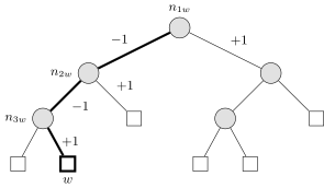
A binary tree over a vocabulary of six words: five internal nodes (grey circles) store the vectors , six leaves (squares) correspond to words. The path to the leaf is highlighted: .
Remark (Why the normalisation is preserved). At each internal node . So at each level of the tree the probability that has come into a node is divided between its two children without loss, and the sum of the probabilities of all leaves equals the probability of the root, that is, one: . The SoftMax denominator no longer needs to be computed.
This contraption is called hierarchical SoftMax: a clever trick that allows us to get rid of computing SoftMax in linear time and to compute it in logarithmic time.
Skip-gram with negative sampling
That was one trick. There is another, substituting the problem. If you ask which of them is used more often in word2vec, then probably the second has after all become more popular; it has become popular in graph analysis too. Let us look at it in more detail. This is Skip-gram Negative Sampling (SGNS). Instead of computing SoftMax, we will set a different problem altogether: we will solve a two-class classification problem; in effect this is logistic regression, where we can make do with sigmoids.
Definition (SGNS: classifying pairs of words into two classes). The log-loss criterion for SGNS (Skip-gram Negative Sampling):
where is the classification model, :
- if the pair of words is in a common context;
- if the pair of words is not in a common context;
- is sampled from in the SG method.
Heuristics and other remarks:
- dynamic window: a random context width ;
- the final word vectors: ;
- the NS (negative sampling) trick is applied when the second class is missing.
How is the functional built? A sum over all the words of our collection, then a sum over all the words in the context of the given word ; this is Skip-gram. Then we build a probabilistic classification model, and we have two classes for pairs of words: either the pair of words is in one context, and we want to predict that, or the pair of words is not in a common context. The first logarithmic term is quite clear to us: it is the logarithm of the probability that the given pair of words is in a common context. But if we used only it, we would have no second class, and we do, after all, have to solve a classification problem. The second class has to be taken from somewhere: we observe the words of the context, but what is a word not in the context? Here the following trick is proposed: we will sample words that are not from the context, but from anywhere, just not from the context of the word . We look somewhere at random and take a random word; that is , that is, we literally sample this word from the collection.
Now a little cheating trick: how to sample. One could sample from the uniform distribution, but that seems bad: there are very frequent words and very rare ones, and it would seem that one should sample with probability , simply the frequency estimate of the probability of the word appearing in the collection. But no such luck: it turns out that a good heuristic is to sample from the distribution , that is, we increase the small probabilities a little. Why exactly three quarters, why not 0.73 or 0.69? Well, it is a heuristic. One could probably play with this parameter, and it would affect the final result somehow, but Tomáš Mikolov apparently ran a series of experiments, three quarters fitted, and ever since everyone has used three quarters.
Now we understand how to solve this problem: by the stochastic gradient method, and for each word position we take the words from the context and also sample a random word not from the context. Since we sample from anywhere, the most diverse words come up as words not from the context in the course of the iterations of the stochastic gradient.
What other successful heuristics are there? The random window size heuristic. What does it lead to? Simply to the words located closer to being chosen more often on average. It is a way of introducing a weighted neighbourhood, so that the weights of the context words decrease with distance from the centre of this context.
There is also a big story: people did many experiments, argued a lot, broke many lances over what to do with the vector representations of the two types. We have built vectors for a word in the role of the predicted one and for a word in the role of the predicting one; then we want to use the vector representations of words, for example, for text classification, for segmentation, for finding synonyms, there are heaps of different applications. Which of the two representations to use? A funny answer: let us just take them and average them with some coefficient .
And one more little question arises: what to do with words that occur for the first time? In some places this is not a problem: there is a good collection of texts, it does not grow, it is known in advance, and we work with a fixed vocabulary. But unfortunately, in text analysis one often has to work with collections that keep growing: news, patents, scientific publications, and social networks, of course. New words may keep appearing; moreover, they may appear because of typos, and for user-generated content this is a very pressing problem. We will come back to this problem a little later.
The connection of word2vec with matrix factorisations
Now let us look at this problem from a slightly different side. There is a fact that was not realised at once: about a year after Mikolov's first paper, a paper by Omer Levy and Yoav Goldberg appeared that explained that in fact Skip-gram and CBOW are merely certain ways of solving a matrix factorisation problem. Strangely enough. Let us see where this comes from.
Theorem (The connection of word2vec with matrix factorisations). Let be the dimension of the word vectors and ; the matrix of the predicting word vectors; the matrix of the predicted word vectors.
SGNS builds a matrix factorisation of the Shifted PMI (Point-wise Mutual Information) matrix:
where is the frequency of the pair of words in a window of words; , are the numbers of pairs involving the word and the word respectively; is the number of all pairs of words in the collection; is the number of negative examples per pair from the context.
As a heuristic, Shifted Positive PMI is also used:
O. Levy, Y. Goldberg. Neural word embedding as implicit matrix factorization. 2014.
We build vector representations of words in two roles, the predicted and the predicting one; we have two matrices, and . And it turned out that Skip-gram Negative Sampling in fact tries to represent as a matrix factorisation the product of these two matrices of vector representations. What does the product of these two matrices mean? We get a "words by words" matrix, where each cell contains simply the scalar product of the two corresponding vectors: for one word and for the other. And it turns out that the SGNS formulation is nothing other than a matrix factorisation of this form.
And what are we factorising? A quantity connected with the frequency of co-occurrence of two words, connected in a slightly strange, but in fact very interesting and correct way. Look: is the frequency of the pair of words in a window of . How to compute it? Run a sliding window of width over the whole body of texts and see how often the pair of words occurs in these windows. Then we compute separately the frequency of pairs involving the word and the frequency of pairs involving the word , and reason as follows. If the appearances of the words and were independent of each other, the frequency estimate of the joint probability would be approximately equal to the product of probabilities ; the cancel there, and in the end we get this formula. If its value is large, that is, is much greater than , it means that these two words go in a pair with each other often not by chance. "By chance" is as if we had shuffled all the words in the text at random: then and would fall next to each other in one window with probability . And if in a real natural-language text, where the words are not rearranged, two words occur together too often, it means that there really is some semantic connection between them: they are close to each other in meaning, or at least there is that very syntagmatic similarity between them.
It is for such a matrix that we in effect build the matrix factorisation , an approximate one, naturally: a low-rank matrix factorisation is unable to describe the matrix exactly, but it can approximate it. There is also this heuristic: to make a positive cut-off. Why? Negative do not interest us at all: these are cases where the words and turn out to be next to each other purely by chance and are in no way connected with each other. So the matrix can be made sparse and these pairs of words not taken into account at all.
Remark (A question: what is). is, in essence, the logarithm of a ratio of probabilities. Let us divide the numerator and the denominator of the fraction by . In the numerator we get , the frequency estimate of the probability that two words appear next to each other. In the denominator, , the frequency estimate that the word occurred, multiplied by , the probability that the word occurred; multiplying these probabilities, we get an estimate of the probability that the words and occurred next to each other purely by chance. For example, words of the general vocabulary will often occur together even after we randomly shuffle the order of all the words in the text, simply because they are frequent in themselves. We have to remove this frequency effect and single out precisely those pairs of words that occur together much more often than if they occurred purely by chance. That is what this construction is for.
What word vectors are for and how they are checked
Now the question: we have built vector representations of words, but why is this done at all? For many reasons: a great many problems can be solved with the help of vector representations of words. In effect we have done a vectorisation: we took a collection of texts, fully unsupervised, with no markup, no teacher marking up words close in meaning, simply took a raw body of texts and assigned a vector to each word. Remember, the lecture before last we talked about recurrent networks for text analysis? A recurrent network at each iteration takes the next word as a vector, and we did not specify then where this vector comes from. Here is the answer: one of the ways of building such vectors in order to feed them to the input of neural network algorithms, in particular recurrent neural networks. Moreover, such algorithms are easy to make pre-trained: one can form pre-trained collections of word vectors, and then people will use them to solve their own problems. This is a very widespread practice.
How is it customary to check how far vector representations of words really reflect the meaning of words? There is a very well-known construction, surely everyone has heard it: "king minus queen equals man minus woman". There are other such foursomes; they are called semantic analogies of words: if you are given any three of these words, you predict the fourth, and this has to be done with fairly good accuracy. More examples of association tasks: a country is associated with its capital, or a country with the name of its currency. There are quite a lot of such examples, test collections have been formed from them, and one can compute how well vector equalities of the type "king − queen = man − woman" work for you, how many errors they make in guessing the fourth word.
Semantic analogies of words (slide): masculine and feminine, the tense of a verb, country and capital.
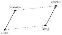
A semantic analogy of words: . Given three words, the fourth is guessed as the one nearest to the vector .
But later this task was criticised. On the one hand, it was a very hyped task; Tomáš Mikolov's 2013 paper is very highly cited, literally everyone who works in text analysis read it carefully, and it proposed this way of checking. A few years later this way was very harshly criticised at computational linguistics conferences, and it was shown on more extensive collections that it does not work all that well. The example is an advertising one, very beautiful and telling, but, first, it is by no means an end in itself: there is no value in the word analogy task as such. It is just an indirect check that the word vectors really reflect the meaning of words so well that vector operations on words lead to a meaningful, interpretable result. It cannot be used directly. Usually vector representations are needed, after all, for solving some pragmatic problems: text classification, segmentation, finding similar words, word sense disambiguation and so on, a great many different applications. It is these problems that have to be solved, and it is on them that numerical quality criteria have to be looked at.
The FastText model
Remember, I said that a question arises: what to do with new words, what to do with words with typos? In 2016 a great paper appeared, and this method, FastText, is still considered one of the best methods for vector representations of words.
Definition (The FastText vector representation model). The idea: the vector representation of a word is defined as the sum of the vectors of all its character -grams :
In Skip-gram, the vectors are trained instead of the word vectors .
Example: , where and are the markers of the beginning and end of the word.
Advantages:
- this solves the problems of new words and of words with typos;
- it is suitable for processing social media texts;
- the vocabulary of 2- and 3-grams is usually smaller than the vocabulary ;
- many pre-trained models exist.
P. Bojanowski et al. Enriching word vectors with subword information. 2016.
The idea is this: let us initially assign vectors not to words but to character n-grams, that is, to pieces of words. Here, for example, is a newly coined Russian word, «дармолюб» (made of two roots, roughly "a lover of freebies"): someone came up with it, many people liked it, and people began to use it actively. If we never had such a word, it was not in the vocabulary, we still want to guess somehow what meaning it may have. In principle it can be guessed, because it is a compound word of two roots, and if we split it into character n-grams, it seems that some meanings remain in these n-grams. The question is whether the vector of a word, that is, the meaning of a word, can be recovered from the vectors of these character n-grams.
What else is remarkable about character n-grams? Their vocabulary is bounded. If a language has, say, 30 letters, then there are no more than trigrams; that is a small vocabulary. Real vocabularies of words can reach millions, while here we have bounded ourselves from above by the number 27 thousand, a very modest vocabulary size. And we require that the vector representation of a word always be made up of the vector representations of its character trigrams. We will train the vector representations of the trigrams so that the vector representations of words made up of them optimise the SGNS criterion well. That is, we are now building a more complex, two-tier model: on the lower tier are the vector representations of character trigrams, but the requirement on them is that the vector representations of words computed from them should predict pairs of words in texts well. This solves the problem both of new words and of words with typos: one can take raw data from a social network with all the delights it contains, pass it through FastText, and a sensible result will come out. And here too there are many pre-trained models with ready-made vectors: FastText was trained on Wikipedia, on news collections, on texts from the internet and so on; there are very many resources where models are already pre-trained for different languages, and they can be taken and used directly for one's own problems.
From texts to graphs
The hype did in fact arise in 2013 after Mikolov's paper appeared, but distributional semantics is a concept known since the middle of the twentieth century. People tried to build vector representations of words by many different methods long before Mikolov: in the seventies and eighties the principal component method was used for this; a great many different attempts were made. Why, then, did this topic take off so strongly precisely in 2013? It simply turned out to be a good and needed paper at the right moment in time. In its wake came a huge number of diverse vector representations: paragraph2vec, doc2vec, sent2vec, this same FastText, StarSpace and many others.
And people realised one simple thing. What are we actually doing? We are building a graph on words. We do not really need the text as a sequence of words: the main thing we do is study the frequency of pairs of words and try to predict high, anomalously high frequencies for some pairs, those that go together in the same contexts. In this way we passed from a linear representation of a text to a representation as a graph: the nodes of this graph are words, and the links correspond to words that appear in the same contexts often, not by chance; a large means that there is an edge of the graph between the vertices and . All methods of the word2vec type and their kin are in fact not about texts but about graphs. As soon as people understood this, they began to transfer these methods to a much broader class of problems, because graphs can model not only texts but also chemical formulas, social networks, recommender systems and a huge number of other applications. So let us now talk about graphs.
Multidimensional scaling
The multidimensional scaling problem
The first problem in this series is in fact also very old: multidimensional scaling. The problem is this: a finite set of points is given, and you know the distances between them. You want to draw these points on a two-dimensional plane so that the Euclidean distances on the plane correspond as accurately as possible to the originally given ones. That is, you are given a finite point configuration in a metric space, and you want to project it into a two-dimensional Euclidean space. Clearly, in the general case this cannot be done without distortions.
In terms of a graph: the points are the vertices of the graph, the edges are the distances. The graph may be complete, when the distances between all pairs of vertices are known, but it may also be that only some of the distances are known; then the graph is not complete, some edges are there and some are not. How to define these distances depends on the problem. In some problems the length of the shortest path in the graph is taken as the distance, and then we really are analysing the structure of this graph. And sometimes the distances simply come from the applied problem: for example, the vertices of the graph are the customers of an online shop, and the distance is how similar the sets of their purchases are. This is already a representation of data for recommender systems; we will talk about them later, there will be a special lecture.
Definition (Multidimensional scaling (MDS)). Given: , a sample of edges of a graph ; , the distances between the vertices of an edge . For example, is the length of the shortest path in the graph (IsoMAP).
Find: vector representations of the vertices such that close vertices (in the sense of a small ) have close and .
The stress criterion:
where is usually the Euclidean distance; are weights: the large distances matter more () or the small ones ().
It is usually solved by the stochastic gradient method (SG).
I. Chami et al. Machine learning on graphs: a model and comprehensive taxonomy. 2020.
We are required to find vector representations of the vertices in a space of, as a rule, not very high dimension; if it is a matter of visualisation, the dimension of the space is two, and we need to lay out the vertices on the plane so that vertices close in the graph have close vectors. The criterion optimised here is customarily called stress; it is a very old name. One of the formulations of the problem: find vector representations of the vertices such that the ordinary Euclidean distance between them corresponds as accurately as possible to the originally given distance ; these are our input data about pairs of vertices.
The small subtlety is that the weights here can be set in different ways. The weight can be made one (), it can be made equal to (), or to (): it all depends on what picture you want to get, whether to preserve large distances more accurately or small ones. The question is non-trivial: distortions are inevitable, and you have to decide whether you want the picture to represent the global structure of the graph well or the local one. If the local one, you should increase the weight of small distances, that is, take ; if you want to represent far distances well and see the global structure, put , and then large distances will have a large weight.
How to solve such a problem? The recipe is fairly universal: use the stochastic gradient method. The parameters here are the vector representations, that is, the matrix : for each vertex a -dimensional vector has to be found. Finding the gradients with respect to them and making gradient steps is not difficult; it is a matter of technique, and I will not go into the technical details here.
Multidimensional scaling for data visualisation
Remark (Multidimensional scaling for data visualisation). With the sample is projected onto the plane.
- It is used to visualise cluster structures.
- The shape of the point cloud can be tuned by the weights and the metric.
- The drawback: distortions are inevitable.
- The most popular modification of MDS is t-SNE.
L. van der Maaten, G. Hinton. Visualizing data using t-SNE. 2008.
Projections of a sample onto the plane with by two methods of multidimensional scaling (slide): the shape of the point cloud depends on the method, the weights and the metric.
What do we get, roughly, with ? As a rule, any such algorithm has some parameters, and for different values of them one and the same data sample is represented in completely different ways. Moreover, the representation may depend on the random initialisation: running gradient descent in different ways, you can get completely different pictures. And they will always be distorted: close original points may turn out to correspond to points that are not close in the picture, and vice versa. There are very many methods, and the most popular can be said to be the t-SNE method. Let us look at it in more detail, because it really is used often, and not only for visualisation but in general for synthesising vector representations of graphs. There are two methods: one is called SNE, the other t-SNE. Let us begin with the simpler one; historically it was the first.
Stochastic neighbour embedding (SNE)
This is Geoffrey Hinton's 2002 paper, Stochastic Neighbor Embedding. The name is very hard to render in Russian, especially if one does not know that embedding is rendered as "vector representation"; one could say "a probabilistic vector representation of neighbourhood". Everyone says "SNE".
Definition (A probabilistic model of the vector representation of neighbourhood (Stochastic Neighbor Embedding, SNE)). Given: original points , .
Find: points on the projection map , , .
Criterion: the distances are close to the original .
A probabilistic model of the event " is a neighbour of " based on renormalised Gaussian distributions:
where is the operation of normalising a vector.
Maximisation of the likelihood (by stochastic gradient):
The original points are vectors in . From them, of course, the pairwise distances can be computed; for some reason in this method it is customary to consider that it is the vectors that are given, although only the pairwise distances between them are used, and the themselves appear nowhere except in Euclidean distances. Next we look for the projection points in a space of low dimension, much less than ; in Hinton's paper this projection is called a map. The criterion: the distances on the map should be close to the original distances, and both kinds of distances are Euclidean.
And here is a completely unexpected trick that was invented in SNE: nobody had done it this way before. To solve multidimensional scaling problems people used the stress functional, even the principal component method, and all these techniques were developed around the sixties and have long been known. And suddenly Hinton comes and says: there are very many imbalances in this problem, so let us turn it into a probabilistic problem, where the probability will estimate that one point is a neighbour of another. It was a very unexpected idea and an unexpected way of attacking the problem, and it turned out to be very successful.
So we build a probabilistic model of the event "the point is a neighbour of the point ", and in two spaces at once. In the original space we introduce a proximity function, a decreasing function of distance, a kernel; it can also be seen as a radial Gaussian; and we also normalise it. Note: the normalisation is over the points : we fix the point and take all the other points except it, that is, the normalisation is over points. After this normalisation we get , a discrete probability distribution whose sum over all equals one. This construction gives an estimate of the conditional probability that is a neighbour of .
Note that for each point we are entitled to choose its own variance . In this lies another very important trick that Hinton came up with: one has to remove the imbalance connected with some points having many neighbours nearby and others few. The heuristic is very much like what happens in nearest neighbour methods; let us recall the first lectures of last semester. There is the Parzen window method, where around each point we fix a constant radius, the same for all points; this works poorly, because one point has a dense neighbourhood and another an altogether empty one. But if we take the distance to the -th nearest neighbour, we get windows of variable width around each point. We are going to do something similar here with the help of the variances : choose them so that at each point we see the same number of neighbours. How to do this comes a little below.
A similar conditional distribution is built in the projection space, where are the vectors sought, and the optimisation will be over them. Now we have two distributions: , given as it were, empirical, fixed, which can be computed from the original data; and , the model one, since it depends on the parameters of the model, the vectors . How are such probabilistic models built? One should use the maximum likelihood principle. The paper, it is true, speaks of minimising the KL divergence, one can speak of cross-entropy, but it seems to me more natural, and we are used to it, to say that we are bringing the model distribution closer to the empirical one by the maximum likelihood principle. These are simply three equivalent ways of naming this criterion.
Perplexity
Remark (The advantages of the SNE method).
- Converting distances into probabilities removes the imbalances between large and small distances.
- The imbalance between points with a high and a low density of neighbours is evened out by tuning by perplexity.
is the entropy of the distribution ; is the perplexity = "the effective number of neighbours of " (if , then ); usually perplexity = 5..50.
The choice of perplexity may substantially affect the look of the projection.
G. E. Hinton, S. T. Roweis. Stochastic Neighbor Embedding. 2002.
Now about how the variances are determined, what it means to tune them. Here a notion from information theory comes to our aid. Let us compute the entropy of the distribution for each point by the well-known formula. Now, there is a quantity, 2 to the power of the entropy, called the perplexity. What is it? It is the effective number of neighbours. Why? Raise 2 to the power of the entropy, taking a uniform distribution: let , that is, the nearest neighbours have equal probabilities and all the others zeros. It turns out that the perplexity is nothing other than this very number of neighbours . So if we want to fix the number of neighbours, we must fix the perplexity of the distribution , that is, its entropy, and tune the variance so as to get the value of entropy or perplexity we need, it does not matter which. That is the way in which we will determine the variances . This can be done by a simple one-dimensional optimisation, for example by bisection, because is monotonically related to the value of the perplexity: literally find the root of the equation, that is, the that ensures the perplexity value we need. It is usually recommended to take the perplexity somewhere in the range from 5 to 50: it is the effective number of nearest neighbours, and for each object.
By tuning the variances, we have balanced all the neighbourhoods in this way: now, in terms of the distributions , each point has roughly the same number of neighbours. Thanks to this balance it is easier to tune the distributions , which depend on the parameters sought.
An original sample of two clusters and its maps at perplexity 2, 5 and 30 (slide).
The figure shows what maps in a two-dimensional space built at different perplexities may look like. Perplexity 2 says that each point has two neighbours on average, and the points spread out like this, moved away from each other; then perplexities 5 and 30. This was an experiment on synthetic data: we knew the ground truth, that is, what the original sample looks like, and one can see that it is possible to choose a perplexity at which we see this sample adequately in the projection too. But this shows, in particular, that the perplexity parameter is very sensitive: depending on how we tune it, completely different results come out. Here the cluster structure of the original data is very simple, just two clusters of points, but at a small perplexity we see a heap of spurious cluster structures that do not actually exist. We might say that there are some interesting structures in the data, while in fact they are artificial artefacts of the method itself.
t-SNE
The last point: how t-SNE differs from SNE. It corrects several drawbacks and allows projections to be made even better; it differs by two improvements.
Definition (The probabilistic model of t-SNE: two improvements of SNE). The crowding problem in SNE: a neighbourhood holds many more points in an -dimensional space than in a -dimensional one.
- Using Student's -distribution, with a heavier tail, and a symmetric joint distribution :
- Using a joint distribution :
Maximisation of the likelihood (by stochastic gradient):
L. J. P. van der Maaten, G. Hinton. Visualizing data using t-SNE. 2008.
Look at the functional: it has the model distribution and the empirical distribution . Originally, in the 2002 paper, it was proposed to build both on the basis of Gaussians, both in the multidimensional -dimensional space and in the low-dimensional projection space. And Gaussians have a very fast decay of the tail. This leads to the model being estimated poorly: if points are far apart, they have a very small probability , and we begin to penalise these points very heavily. To prevent this, one has to raise the tails of the model distribution.
There is one more motivation for doing this: the model distribution lives in a space of low dimension, and the original points in a space of high dimension. Hence the crowding problem: when you have a neighbourhood of neighbours in the original multidimensional space, it is very hard for you to embed these neighbours into a two-dimensional space, and they form this crowding. To prevent this, for the model distribution we take not the Gaussian distribution but another one, with heavier tails, for example Student's distribution with one degree of freedom; the formula has changed a little. By the way, all these formulas have very compact expressions for the gradients: when the gradients are derived analytically, it turns out that both for Gaussians and for Student's distribution very efficiently computable simple expressions are obtained.
The density of the normal distribution (blue) and of Student's distribution with one degree of freedom (red) (slide).
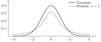
The density of the standard normal distribution and of Student's distribution with one degree of freedom . The second has much heavier tails: far-apart points on the map do not get a vanishingly small probability .
What is the interesting feature of t-SNE? The authors, under Hinton's supervision, thought very well about how to formalise the loss function correctly so as to get rid of all those imbalances, skews and distortions that usually haunted multidimensional scaling methods. One can say that it is an advanced multidimensional scaling built on an analysis of why the ordinary loss functions, quadratic ones of the stress type, did not fit.
Remark (A question: why the joint distribution). The second improvement is symmetrisation: instead of the conditional distributions and , the joint distributions and are used. The motivation here is this: with such expressions the gradients are easier to compute, the expressions come out simpler. I will not write this out; one can look at how it is done in the papers.
Remark (The advantages and drawbacks of t-SNE).
- A better representation of similarity structures compared with other multidimensional scaling methods.
- False cluster structures at low perplexity.
- It is hard to tell real structures from artefacts of the method.
M. Wattenberg, F. Viégas, I. Johnson. How to use t-SNE effectively. 2016. https://distill.pub/2016/misread-tsne
Maps of a sample of handwritten digits (mnist) by three multidimensional scaling methods (slide): graphviz, LinLog and t-SNE.
Vector representations of graphs
Matrix factorisations
It remains to talk a little more about vector representations of graphs. Multidimensional scaling is in fact not the only approach to obtaining vector representations of the vertices from information about the edges of a graph. Another way is connected with the matrix factorisations that we have already mentioned today.
Definition (Matrix factorisations (graph factorization)). Given: , a sample of edges of a graph ; , the proximity between the vertices of an edge . For example, is the adjacency matrix of the vertices.
Find: vector representations of the vertices in such that vertices close (in the graph) have close vectors.
The criterion for an undirected graph ( is symmetric):
The criterion for a directed graph ( is non-symmetric):
It is usually solved by the stochastic gradient method (SG).
I. Chami et al. Machine learning on graphs: a model and comprehensive taxonomy. 2020.
On a sample of edges of a graph some information about the proximity between vertices is given. For example, it may be the adjacency matrix of the vertices, that is, a 0–1 matrix where a one stands for those pairs of vertices that are joined by an edge. But it may also be a matrix of weights, of some proximities between vertices: the larger the proximity value, the smaller the distance between the vertices. The problem is again to find vector representations of the vertices such that close vertices can be predicted from them. This is the problem of predicting the presence of a link in a graph (link prediction), and it has very many applications in the most diverse fields. For example, recommender systems: there are people vertices and item vertices, and items have to be recommended to people; or a social network, where people can be recommended to people.
The problem is solved in a very similar way, only instead of distances scalar products are used: the scalar product of the vector representations of two vertices is directly suitable for predicting proximity. In principle one could put some link function here, for example a sigmoid, some nonlinear function of the scalar product, but usually people do not bother and do it more simply.
Two cases are distinguished. When the graph is undirected, an edge has no arrow, no beginning and end; two points are simply joined to each other. Then the matrix is symmetric, and one can use the same vector representation for both the incoming and the outgoing vertex: the factorisation is built. If the graph is directed, one has to deal with a non-symmetric matrix , and the matrix factorisation is non-symmetric too: you have two different matrices, and you build the matrix product , in which both matrices are unknown but must approximate the known matrix. This problem too is usually solved by the stochastic gradient method.
Random-walk models: DeepWalk and node2vec
One more interesting idea. We have understood that a text is a graph that represents the syntagmatic similarity of words. What does the Skip-gram model do with a text? It takes each word and considers its neighbourhood; the neighbourhood contains words close to it in meaning, and then the work goes on with these words. Now let us forget that this is a text and consider that we have not words but vertices of a graph. What changes? By and large nothing, but then we have to define what the context of a vertex is. In a text it was clear: go five words to the left, go five words to the right. Here the situation is more complicated. If we are at a vertex of the graph, it is in principle clear that the nearby vertices joined by edges are, as it were, the context. But in many problems one wants to go farther and look at vertices connected not by one edge but through two edges, through three and so on, that is, to look at a deeper neighbourhood of the given vertex. The problem is that if the graph is strongly connected, the size of the neighbourhoods grows exponentially: the second and third neighbourhoods will already be huge in volume. But the same idea of sampling comes to the rescue: the context can be generated by a random walk. When we use stochastic gradient on a text, we run over the words in a row. On a graph we choose some vertices at random and then from each vertex we pass at random through its neighbourhood, and this neighbourhood too can be built by a random walk.
Definition (A random-walk model for large graphs). Given: , a sample of edges of a graph .
Find: vector representations of the vertices , .
The criterion for the probabilistic model :
where is the neighbourhood ("context") of the vertex , sampled by a random walk of length (DeepWalk, node2vec); are vertices far from , sampled as .
Parametrisation of the random walks: the probability after the transition ;
- , : closer to breadth-first search (BFS);
- , : closer to depth-first search (DFS).
B. Perozzi et al. DeepWalk: online learning of social representations. SIGKDD-2014. A. Grover, J. Leskovec. Node2vec: scalable feature learning for networks. SIGKDD-2016.
Otherwise it is the very same Skip-gram Negative Sampling that came from texts: the probability that there is a short path from the vertex to the vertex is modelled by a sigmoid of the scalar product of the vectors, the vertices from the context give positive examples, and the far vertices, sampled with the same power , negative ones.
There is a very good method called node2vec; it was made two years after DeepWalk. DeepWalk simply walks over the neighbourhood somehow at random, while node2vec parametrises this way of traversal, and in a rather interesting way. It says: we do not know what we need, depending on the subject area and the problem, whether depth-first search or breadth-first search. Let us parametrise the probabilities with which we pass from one vertex to another so that, depending on the value of the parameter, we get either an immediate departure far from the vertex into the depths, which is depth-first search, or circling around one vertex, which is then breadth-first search.
The parametrisation of the random walk in node2vec (slide): the walk came from to ; the weights of the next step are , , .
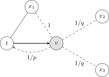
The parametrisation of the random walk in node2vec: the walk has just passed from to . The unnormalised weights of the next step: return to (distance 0 from ), ; go to , a neighbour of (distance 1), ; go off to or (distance 2), .
This is done very easily. Suppose we first stood at the vertex , then passed to the vertex , and now we have a dilemma. With the next move we can get either back to the vertex , the distance from being zero; or to a vertex that has a link with , the distance being one; or to a vertex that is connected with only through two edges, distance two. For each of these three cases one simply has to specify a probability of its own, and this is done with two parameters. If we take as one the chance of going to a vertex at distance 1, that is, connected with , then the chance of returning to is , and the chance of going off one more edge is . These and are the two parameters with which one can set a compromise between going deep and going wide. Such a parametrisation of random walks allows one to explore either long neighbourhoods or the neighbourhoods of only the very nearest neighbours of a vertex.
Graph autoencoders
A reminder: autoencoders for semi-supervised learning
And the last, but probably the most important thing in this lecture. I want to remind you from the last lecture what an autoencoder is: we will now draw a connection between everything I have told about vector representations of graphs and autoencoders.
Definition (Autoencoders for semi-supervised learning (a reminder)). Data: labelled , unlabelled .
Find three models:
- , the encoder;
- , the decoder;
- , the predictor.
Loss functions are given: , the reconstruction; , the prediction.
Criterion: joint training of the autoencoder and the predictive model (classification, regression or other):
D. Bank, N. Koenigstein, R. Giryes. Autoencoders. 2020.
An autoencoder for semi-supervised learning (slide): the encoder , the decoder and the predictor use a common vector representation .
If we have a sample of objects, let us call them unlabelled, then an autoencoder is usually the optimisation of this quality criterion. We have an encoder with parameter , by which we build a vector representation of the object ; a decoder with parameter restores, reconstructs, the object , and the reconstructed should correspond as well as possible to the original . This correspondence is described by a loss function that evaluates the quality of the reconstruction of the object by such an "encoder–decoder" pair. If we speak of neural networks, the encoder may be a fully connected network, a convolutional network, it does not matter; very many different architectures can be used here. The main thing is that the encoder translates the original object into a vector description of a given dimension, and the decoder restores the original object and tries to do so as accurately as possible.
What are autoencoders actually needed for? To solve some useful problems with the obtained vector representations , for example classification or regression. Then we already have a ready feature description for these problems: the original object may be inconvenient, complexly structured, of too high a dimension, and with the encoder we have compressed it into a vector representation, in effect generated features, done feature generation. These generated features can be fed to the input of a classifier, a regression or another machine learning model that initially works well with vectors. Naturally, this second problem also has its own loss function . And since the feature descriptions fed in here are the output of the encoder, it turns out that in the two problems part of the parameters, namely the encoder's parameters , are common. So it is better to train them jointly.
There are, in fact, two strategies. One is dumb and outdated: first build an encoder–decoder pair on the unlabelled data, without looking at anything, get the vector representations of the objects, and then drive them into some classification method and solve the problem with these hidden representations. A two-stage scheme in which the stages are in no way connected with each other, despite their having a common parameter . So a good idea is to combine the two stages into one and get a joint optimisation problem, where the parameter will be optimised taking two problems into account at once. The first is to build good reconstructions: we require of the vector representations that they preserve the full information about the original object as far as possible, as far as the dimension of the vector allows, that is, that be as informative as possible; this is achieved by the "encoder–decoder" pair. The second is the problem that interests us business-wise, for example a supervised predictive model: we have a special labelled sample, that is, we are also in the setting of semi-supervised learning, and from these labelled data we want to build a good classifier. But the classifier will be good if the vector representation is good and tailored to solving this problem: it is not only as informative as possible thanks to the autoencoder, but must also solve this problem well. That is, these are not just any features that characterise the original objects well, but features that are as well suited as possible to the classification model, to solving the problem on the labelled sample. A joint optimisation of the parameters , and is needed, where are the parameters of our classification model. A very good idea: build two models at once.
Vector representations of graphs as autoencoders
Now a really cool mega-generalisation of this idea, which I read in one paper, a really great 2020 survey of models on graphs. Let me lead up to the motivation. Let us look back once more at the methods of vector representations of graphs that we have seen today. There were three of them.
Multidimensional scaling: at the input, information about the distances between vertices; at the output, vectors whose Euclidean distances should correspond to the original ones. SNE and t-SNE: at the input, the same distances between objects, which we recomputed into proximities, and the proximities into the probability of being a neighbour; from this probability we build a probabilistic model of being a neighbour, and this model depends on low-dimensional vector representations of the objects. Matrix factorisations: at the input, distances or an adjacency matrix, that is, how the vertices of the graph are connected by edges, and we build vector representations of the vertices so that their scalar products correspond well to the original data about the edges.
What do these three stories have in common? That numerical information about the edges of a graph is given, and we build vector representations of the vertices of the graph that allow the information about the edges to be reconstructed well. I deliberately used the word "reconstruct" so that you realise: this problem is insanely similar to the one autoencoders solve. Only the autoencoders we are used to work with objects and restore information about objects, while here I am claiming that we are working with autoencoders that build vector representations for objects, the vertices of the graph, but restore information about the relations between these vertices, that is, about the edges. That is the whole conceptual modification.
Remark (Vector representations of graphs as autoencoders). All the methods of vector representations of graphs considered above are autoencoders of the data about the edges:
- multidimensional scaling: ;
- SNE and t-SNE: ;
- matrix factorisations: or .
The encoder's input: , the data about the edge of the graph. The encoder's output: the vector representations of the vertices . The decoder's output: an approximation computed from .
I. Chami et al. Machine learning on graphs: a model and comprehensive taxonomy. 2020.
In essence, everything we said about multidimensional scaling, SNE, matrix factorisations and ways of vectorising graphs is autoencoders: the data about the edges go to the encoder's input, at the output it gives vector representations of the vertices, and the decoder approximates the data about the edges by looking at the vector representations of the vertices. Structurally this is an autoencoder.
GraphEDM: a generalised autoencoder on graphs
So, the promised generality. I liked this 2020 survey paper very much, because in it the authors proposed a certain scheme and showed that it generalises some 30 different models of vector representations of graphs, graph neural networks and so on. It turns out that they all fit into one common scheme, which we will now look at, and it will be very clear, because it is simply an analogue of the scheme of an autoencoder for semi-supervised learning that we have just recalled.
The generalised autoencoder on graphs GraphEDM (slide).
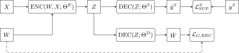
The generalised autoencoder on graphs GraphEDM. The encoder builds the vector representations of the vertices from the data about the edges and about the vertices ; one decoder solves a supervised problem, and its output is compared with the labels ; the other reconstructs the data about the edges, and its output is compared with the original (dashed).
Definition (GraphEDM: a generalised autoencoder on graphs). The Graph Encoder Decoder Model generalises more than 30 models:
- , the input data about the edges;
- , the input data about the vertices, feature descriptions;
- , the vector representations of the vertices of the graph;
- , the decoder that reconstructs the data about the edges;
- , the decoder that solves the supervised problem;
- , (semi-)supervised data about the vertices or the edges;
- , loss functions.
I. Chami et al. Machine learning on graphs: a model and comprehensive taxonomy. 2020.
The difference from the scheme for ordinary objects is only that in the case of graphs the input data may be of two types. First, as before, information about the original objects, which may be in the form of feature descriptions of the vertices . Second, information about the edges, some matrix . Earlier we had different notations for it, , , , and now we say that all this is input data about the edges and denote it .
What does the encoder do? It forms vector representations of the vertices, and it can use both information about the vertices and information about the edges. This is a general approach that generalises very many different methods: some take only , others only , still others can take both. Next, what are these vector representations of the vertices needed for? For two problems. The first is supervised: we have labelled data, and we want to predict something about the vertices or about the edges; here too there are two variants, two different formulations of problems. The main thing is that is used as vector feature descriptions, outputs are formed from them, and we compare these outputs with the labelled information by a loss function. Thanks to this, is tuned to solve this problem well. The second problem forces to be a good vector description; it is the reconstruction problem, exactly as in autoencoders: from we must be able to reconstruct . The dashed line is drawn here precisely to show that the loss function compares the reconstructed with the original . In this way we force to be as informative as possible.
And it turns out that this scheme is very universal: the joint solution of two problems, a supervised one and an unsupervised one that reconstructs information about the edges of the graph. This concept has proved very general. It seems to me it will be very useful, if you ever come across problems on graphs, whatever you will be doing, chemical compounds, recommender systems or anything that has a graph representation, to remember this paper, and the floor is yours: it is a very general and, it seems, very correct approach to these problems.
Graph neural networks
And literally the last thing, just a mention, because the topic of graph neural networks has grown insanely in literally the last five or six years; below I give only surveys, four of them, and only from the last two years, on representations of graphs and graph neural networks. As a teaser, one of the ideas considered most productive in graph neural networks.
Definition (Graph neural networks (Graph Neural Network, GNN)). Given: , a sample of edges of a graph ; , the feature descriptions of the vertices ; the labels .
Find: vector representations of the vertices and the parameters of a recurrent network with message passing:
where is the set of vertices neighbouring the vertex ; is the vector representation of the vertex at iteration ; is a multilayer neural network with parameters .
The criterion is that for an autoencoder + a predictive model.
I. Chami et al. Machine learning on graphs: a model and comprehensive taxonomy. 2020. Ziwei Zhang, Peng Cui, Wenwu Zhu. Deep learning on graphs: a survey. 2020. Zonghan Wu et al. A comprehensive survey on graph neural networks. 2019. Jie Zhou et al. Graph neural networks: a review of methods and applications. 2019.
A graph neural network is nothing other than a special case of this general concept. The only difference is that a multilayer neural network is used to estimate the vector representation at each vertex from its neighbourhood. You go over all the vertices in the neighbourhood of the given vertex and use some very complex function , which may be a deep neural network, but the main thing is that its input is the feature description of the vertex, the feature description of its neighbour, the neighbour's vector representation from the previous iteration, and some model parameters. The second function, , which may also be a neural network, is used for the predictions proper, which you will compare with the training sample by means of a loss function. Here the vector representations of the objects extend the original feature descriptions; together they are fed to the input of this neural network, and it makes the prediction. And the first line is merely the encoder. You write out the loss functions on the basis of the substantive meaning of the problem being solved, and this sets the architecture of a very wide class of models. Then an iterative process is started, a bit like recurrent neural networks. There are various modifications: there are that resemble convolutional neural networks, there is a huge number of different architectures there, but that is beyond the scope of today's lecture.
Summary
Remark (Summary). Varieties of data vectorisation:
- autoencoders: synthesis of vector representations (embeddings) of objects, usually with dimensionality reduction;
- matrix factorisations of graph data (GF, graph2vec) and multidimensional scaling (MDS, SNE): synthesis of embeddings of objects from data about their interaction;
- the generalised GraphEDM model: synthesis of embeddings of objects from data about the objects and their interaction.
The training methods are based on SG.
Text data are a special case of graph data:
- words are the vertices of a graph, the co-occurrence of a pair of words is an edge;
- words and documents are the vertices of two different parts of a graph, the occurrence of a word in a document is an edge of a bipartite graph.
To sum up briefly: vector representations, embeddings, are built for complexly structured data, such as texts or graphs. Graphs are the more general representation, texts their special case. If your data are complexly structured but you have managed to describe them by a graph, you understand that you have information about the edges and need to build uniform vector representations for the vertices, then the mechanism told about today is intended precisely for this problem.
No comments yet
Be the first to share your thoughts.