August 30, 2026 · Lecture · LibreTimes
Machine Learning 2. Lecture 2. Neural Networks for Unsupervised Learning
Contents
- What this lecture is about
- Kohonen networks for clustering and visualisation
- The clustering problem and the Kohonen network
- Hard and soft competition
- Kohonen maps
- Interpreting Kohonen maps
- Autoencoders
- The formulation of the problem
- The linear autoencoder and the principal component method
- How autoencoders are used
- The sparse autoencoder
- The denoising autoencoder
- The contractive and relational autoencoders
- The variational autoencoder
- Autoencoders for supervised learning
- The multilayer autoencoder
- Joint training of several models
- Pre-training and transfer learning
- Multi-task learning
- Self-supervised learning
- Distillation and surrogate modelling
- Learning using privileged information
- Generative adversarial networks (GAN)
- Conclusions
- Seminar
What this lecture is about
Today is the second lecture of this semester; we continue studying neural networks, and the topic is methods of unsupervised learning. A very important and interesting topic. To warm up, we will first deal with the clustering problem: unsupervised learning is associated first of all with it. Then, and this is probably the central part of today's lecture, autoencoders: a very important class of neural network models that is now used in very many places; we will run through their main types. And at the end there will again be a run through various modifications of the idea of unsupervised learning, mainly about how to train several models at once. We will see how rich the variety of ways is in which this general meta-idea can be implemented in neural networks, to great benefit for the most diverse problems.
Kohonen networks for clustering and visualisation
The clustering problem and the Kohonen network
Let us begin with a simple reminder of what the clustering problem is and how a simple approach to clustering can be implemented on a neural network architecture. These are rather old things, the so-called Kohonen networks.
Definition (The formulation of the clustering problem. Data quantisation). Given: , a training sample of objects, ; , the Euclidean metric in .
Find: the cluster centres , ; the clustering model is the "hard competition rule" (WTA, Winner Takes All):
Criterion: the mean intra-cluster distance
Data quantisation is the replacement of by the nearest centre .
Let a training sample be given, the objects represented by vectors in , that is, each object is described by numerical features, and the only thing we have is a distance function between objects; we will consider it the Euclidean metric. We are required to find the cluster centres. Recall the lecture on clustering from last semester: the requirements on the clustering problem can be formalised in different ways, and one of the simplest is minimising the mean intra-cluster distance. The parameters of the clustering algorithm are the cluster centres . is a finite set of clusters, and the number of clusters in this problem we set in advance. If we say that we want to split the set of objects into 10 clusters, where did the 10 come from? By and large, arbitrarily; if we do not know it exactly, we will solve the problem many times, experimenting with the number of clusters.
The principle of clustering is very simple: the algorithm assigns the object to the nearest cluster. This is also called the hard competition rule, or "the winner takes all". Who is the winner here? A cluster: it takes for itself the object that turned out to be closer to it. One can also consider it the other way round, that the winner is an object, which takes for itself the nearest cluster; they correspond to each other completely. We measure the intra-cluster distance by the square of the Euclidean metric, the square because we will have to differentiate this criterion. The object has been assigned by the clustering algorithm to some cluster, the centre of this cluster is described by the vector , and we measure the distance from the object to the centre of its cluster; the sum of such intra-cluster distances has to be minimised over the set of vectors for all clusters. As soon as the problem is written out as a criterion to be optimised over parameters, and we have clearly realised what the parameters are, then the stochastic gradient method can be used.
The Kohonen network is a two-layer neural network (slide): the first layer computes the distances to the cluster centres, the second chooses the minimum.
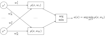
The Kohonen network: the weights are the coordinates of the cluster centres; the first layer computes the distances to the centres, the second, non-standard one, the .
Definition (The Kohonen network (a network with competitive learning)). The structure of the model is a two-layer neural network, .
The gradient step in the SG method for a chosen :
If belongs to the cluster , then moves towards .
T. Kohonen. Self-organized formation of topologically correct feature maps. 1982.
Why does this have anything to do with neural networks at all, where is the neural network here? It may seem a little far-fetched, but in fact it really is a two-layer neural network, where the input elements are the coordinates of the vector . Next we compute the distance between and . Note: if the distance is Euclidean and we agree that the vectors and are normalised, that is, the whole sample and all the parameters live on the unit sphere, then computing the distance is equivalent to computing the scalar product: minimising the distance between vectors is the same as maximising their scalar product. And then it becomes clear that this is a real neural network: the scalar products of the vector with the parameter vectors, the weights of the synaptic connections of each neuron, are computed. And the second, slightly non-standard, layer computes not a sum but the . We are already used to the fact that in neural networks it is not at all necessary to compute precisely a weighted sum in each neuron; other functions may be computed too; we will see many more such examples.
The gradient step of stochastic gradient looks as usual: we pull objects out of the training sample one at a time in random order and for each take this step; if we substitute the Euclidean metric and differentiate, we get exactly this formula. How is it interpreted? If was assigned to the cluster , then the centre of this cluster, the vector , a vector in the same space where the objects live, moves slightly in the direction of the object . The objects are clustered in turn, the nearest centre is chosen for them, and this centre moves slightly towards the object. The cluster centre keeps darting a little between the objects assigned to it, and so ends up somewhere in the middle between them. A very clear learning principle; this formula could have been written out as a pure heuristic, without even turning to neural networks, but here it is obtained in a regular, proper way.
Definition (The SG (Stochastic Gradient) algorithm for the Kohonen network). Input: a sample ; the learning rate ; a parameter . Output: the cluster centres , .
- initialise the centres , ;
- initialise the current estimate of the functional: ;
- repeat
- choose an object from (for example, at random);
- find the nearest centre: ;
- gradient step: ;
- estimate the value of the functional: ;
- until the value of and/or the weights stabilise.
Then we only have to watch the convergence of the process: we initialise the current estimate of the functional, accumulate the current value of the functional by an exponential moving average and watch how it changes with the iteration number, and the convergence criterion says that either the weights have stabilised, the cluster centres have stopped changing, or the functional has converged and also stopped changing substantially.
Hard and soft competition
Definition (Hard and soft competition). The hard competition rule WTA (winner takes all):
The drawbacks of the WTA rule: a slow rate of convergence; some may never be chosen.
The soft competition rule WTM (winner takes most):
where the kernel is a non-negative non-increasing function. Now the centres of all clusters move towards , but the farther from , the smaller the size of the shift.
What drawback does this algorithm have? When the winner takes all, we took one object, found the nearest centre for it and moved it slightly towards the object. It turns out that we will converge rather slowly: for one object we change the centre of only one cluster. One more drawback is that some centres may never be chosen at all: they are initialised randomly, and it may turn out that some has flown off somewhere to the side, not a single object belongs to precisely it, and this centre will stay as it was initialised.
To overcome these two difficulties, the soft competition rule is introduced. We took the object ; it has a nearest cluster, but perhaps there are several clusters to which it is roughly equally close. Why, then, do we change only the centre of the closest one? Let us move all the nearest clusters slightly towards this object, and "slightly" will depend on how far they are from each other. Let us soften the binary expression equal to one on one and only one cluster: introduce a kernel, a decreasing function of distance with values from zero to one. We have seen such a construction more than once: in Parzen density estimates, in nonparametric regression. Here it helps to increase the rate of convergence: all the clusters that turned out to be in the neighbourhood of the object we move slightly towards it.
This looks like a heuristic, like a modification of a ready-made algorithm derived from the requirement to minimise a functional. One may ask whether there is not a functional here too that we are minimising; I will leave that to you as a question to think about: with a little fiddling one can write such a functional out. It is simpler to understand this as a very simple modification of the algorithm. In effect the object belongs to several clusters at once; one can even recompute the proximities into probabilities: the greater the proximity between the object and the centre of a cluster, the more strongly the object influenced this centre. The object is assigned a vector of degrees of membership in all clusters, and this idea may prove productive: you have obtained a new vector representation of the object as a vector of degrees of proximity to each cluster. And this really does speed up convergence.
Kohonen maps
We have talked about two strategies, "the winner takes all" and "the winner takes most", that is, hard and soft clustering. But speaking of Kohonen networks, one cannot fail to mention the so-called Kohonen maps. This is a special case of the same clustering algorithm, and it is used for visualising multidimensional samples. The sample of objects is in a space of dimension , and sometimes one very much wants to see with one's eyes how the clusters are located, how the objects group around them. But an -dimensional space is hard to visualise, and the idea arises: could it not be projected somehow onto a two-dimensional plane so as to show it on a computer screen?
Definition (The Kohonen map (Self Organizing Map, SOM)). Given: a training sample , , .
Find: the cluster centres , , .
Along with the metric on , a metric on the grid is introduced:
Teuvo Kohonen. Self-Organizing Maps. 2001.
The neighbourhood of the node on the rectangular grid of cluster centres (slide).
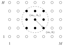
A grid of cluster nodes; the filled nodes are those falling into the neighbourhood of the node of radius 1.5 in the grid metric .
The idea here is rather original and at first sight breaks the patterns, because we did not agree on this before. Now let us agree that we will have as many clusters as there are nodes in a rectangular grid. The grid of clusters is, as it were, a pixel picture: each cluster will now be a pixel, and in each cluster we will depict something by colour. The width of the grid is , the height ; be prepared at once that, since this is a pixel picture, and are fairly large, tens, perhaps hundreds. In each node of this grid I put a cluster centre, a vector of dimension . How many parameters is that in all? We get a three-dimensional cube of numbers: each node of the grid stores an -dimensional vector of the cluster centre.
The sample will be clustered over these clusters, but, unlike what you are used to, here it may turn out that not a single object falls into some cluster, and even that not a single object falls into most of the clusters. The objects, assigned to the nearest clusters, fall, as it were, into points of this pixel picture, but not into every pixel. This has to be realised; it is unusual: usually in a clustering problem quite a lot of objects belong to each cluster, and there are far fewer clusters than objects. With Kohonen maps it may be the other way round: there are fewer objects than clusters, since the number of clusters is the number of pixels in the picture.
And one more unusual thing: besides the Euclidean distance in we introduce one more distance function, also a Euclidean metric, but on the nodes of the grid, the distance between pixels of the picture. Each pixel has a neighbourhood described by this metric: is the node of the grid into which the -th object fell, and an arbitrary node.
Definition (Training a Kohonen map). Input: , the training sample; , the learning rate. Output: , the weight vectors, , .
- , initialisation of the weights;
- repeat
- choose an object from at random;
- WTA: compute the coordinates of the cluster: ;
- for all :
- WTM: take a gradient descent step: ;
- until the clustering stabilises.
Teuvo Kohonen. Self-Organizing Maps. 2001.
The algorithm becomes more complicated at one point. We choose an object from the sample at random, as in stochastic gradient, and by the rule "the winner takes all", hard clustering, compute the centre of the cluster into which the object falls: here the Euclidean distance between vectors in , the object and the cluster centre , which is also a vector from and sits at the node of the grid . Let us denote the node found . And now an unusual thing is done: the clusters nearest to the object we now count not by the metric in but by the metric on the nodes of the grid; that is the neighbourhood. And for all of them we take a gradient descent step by the rule "the winner takes most", soft clustering: all the cluster centres that turned out to be nearby on the rectangular grid we move slightly towards the object , as vectors in . There is a constant duality of representation all the time: on the one hand, each cluster is a node of the grid, and on the other, in the node sits a vector from that can be compared with the objects of the sample. As vectors from we compare them when we determine which node an object will fall into; and as soon as it has fallen into a node, we take the nodes neighbouring it on the grid and move their vectors, their centres , slightly in the direction of the object.
Interpreting Kohonen maps
Remark (Interpreting Kohonen maps). Two types of graphs, colour maps :
- the colour of the node is the local density at the point : the mean distance to the nearest points of the sample;
- one map for each feature: the colour of the node is the value of the -th component of the vector .
Example: the UCI house-votes problem (US Congress voting patterns). The objects are congressmen; the features are the results of voting on various questions; there is a target feature "party" {Democrat, Republican}.
We wanted a two-dimensional visualisation of the cluster structure of an -dimensional sample. Graphs of two types are built, colour maps of size . In the first type, the colour of a node conveys the local density: the mean distance to the nearest points of the sample. We get a smeared picture; it is usually drawn in shades of grey or in a single colour.
The second type is again an original idea. We have a cube: an grid, an -dimensional vector sits in each node, and its coordinates correspond to the features of the objects. Let us take a slice of the cube along the -th coordinate, that is, the value of the -th feature for all the cluster centres. The cluster centres, as vectors from , are similar to our objects; in a sense they are mean representations of nearby objects. The slice along a feature gives a colour map, and such maps are customarily drawn in "geodesic" colours, like geographical maps: blue is the lowest value, then green, yellow, red, brown the highest. The map shows how the values of the -th feature are distributed over the plane, and dots can show how many objects of the sample fell into each node of the map.
An example is a problem from the UCI repository about how American congressmen vote on various questions. The objects are congressmen, the features are binary, the results of voting on particular questions, and there is a target feature, party affiliation: Democrat or Republican; it too can be displayed on the map as one of the features. The problem is fairly simple; there are in fact two clusters in it, and on the map of the first type we see them as lighter areas. On the maps of the first type the overall cluster structure is visible, and on the colour maps of the second type how the values of a feature are distributed in the same plane, and one can give explanations: some clusters are characterised by low values of the feature, some by high ones. The whole visualisation is done in order to see whether there are connections between the cluster structure and the maps of individual features. Looking at all the features of this problem, we see that the two main clusters correspond clearly to the parties: there are Democrats, there are Republicans. And on the bulk of the questions the parties really do vote in unison: many maps are very similar to the distribution by party, that is, on these questions the party has a concerted opinion. In some places the pictures are not similar: for example, on some question there was unanimity, and the parties voted roughly the same way. With one glance at the colour maps one can understand the nature of the clusters: what features they are connected with.
Remark (The practical application of Kohonen networks). A question: could there be some practical example of the use of Kohonen networks?
First, clearly, it is simply a tool for solving the problem of clustering vectors from . Second, Kohonen maps are one of the main applications of Kohonen networks; the example with the congressmen's voting is precisely such an application. Before, in the last lecture and in the last semester, we considered exclusively neural networks for supervised learning: regression or classification. Now we have considered how to solve the clustering problem by a neural network approach, and one of the applications is visualisation.
Remark (The merits and drawbacks of Kohonen maps). Merits:
- the possibility of visual analysis of multidimensional data;
- quantisation of the sample over clusters with automatic determination of the number of non-empty clusters.
Drawbacks:
- subjectivity: the map reflects not only the cluster structure of the data but also depends on the properties of the smoothing kernel, on the (random) initialisation, on the (random) choice of in the course of the iterations;
- distortions: close objects of the original space may pass into distant points on the map, and vice versa.
Recommended only for exploratory data analysis.
The map will depend strongly on what the random initialisation was, and in general a multidimensional space cannot in the general case be represented on a plane without distortions. Distortions can be of any type: points originally close may turn out far apart on the map, and vice versa. So this is not a means of deep analysis but a means of preliminary, exploratory data analysis. The pictures come out beautiful, one can charm the client with them, and in my view this is in general the main function of Kohonen maps: it is fun and beautiful, but not a reliable quantitative method.
Autoencoders
The formulation of the problem
Let us consider that we have warmed up: the clustering problem is something we understand well. Now the second topic, central for today's lecture: autoencoders. Ask questions more actively: if you do not understand the first slide with the formulation of the problem, it will be a big loss. Although there is nothing complicated here; moreover, recall right away what the principal component method and the singular value decomposition are; I will now develop this analogy.
Definition (An autoencoder (AutoEncoder): unsupervised learning). Given: , a training sample.
Find two models at once:
- , the encoder, the code vector ;
- , the decoder, the reconstruction .
Criterion: the quality of reconstruction of the original objects :
The quadratic loss function: .
Example 1. The linear autoencoder: , , , .
Example 2. A two-layer network with activation functions , : , .
Again there is a training sample, just objects, no answers; this is an unsupervised problem, there are no y's. Our task is to build a pair of transformations, an encoder and a decoder, that allow the original objects to be reconstructed. The encoder translates an object from the original space into some new space ; it is simply a function of . For understanding, it is assumed that the dimension of is smaller than that of the original space: we are looking for a new feature description that will encode our objects efficiently. A complete analogy with the principal component method. What does it do? It looks for a low-dimensional projection such that, if the original objects are projected onto this subspace, the bulk of the information about them is preserved: by some inverse transformation the original objects can be restored with good accuracy from the compressed low-dimensional description. In essence this is data compression: vectors from a high-dimensional space are translated into a low-dimensional space so that they can be restored. The restoring transformation is called the decoder; it works from back into , and we denote the reconstructed object .
For the reconstructions really to be good, let us impose a requirement on the superposition: having applied the function to , and the function to the result, we must get something similar to the original , and the more similar, the better. An optimisation problem arises from this at once. Let us introduce parameters: the encoder has a parameter vector , the decoder a parameter vector ; these are two parametric families of mappings, and the parameters and have to be tuned jointly so that the reconstruction is as similar as possible to the original objects. The loss function should characterise how much an object and its reconstruction differ; for example, a quadratic one, and we come to the method of least squares; in effect we have reduced the problem to regression.
An example is the linear autoencoder: a parametric family with a matrix parameter , that is, simply multiplied by . We pass from a space of dimension to a space of dimension , smaller, it is implied. Easy to remember: as in "minor". The matrix is also a linear transformation, to return to the space of the original dimension. One can bring this little model closer to neural networks by adding a small nonlinearity: a free term, the vector , and an activation function, for example a sigmoid or ReLU. Then the superposition becomes a two-layer neural network; this is the neural network generalisation of the linear autoencoder.
Remark (Invertibility and the loss function). A question: do we impose on and a requirement of invertibility in the mathematical sense?
Generally speaking, no. The optimisation problem is a general one: it will pull out the parameters and , and we will get particular transformations, and how well they will work depends on how rich the family of functions taken is, whether there are enough parameters to set up the forward and the inverse transformation. Inverse, naturally, in quotation marks: it is approximately inverse, it approximates the inverse transformation, because as a rule we do not reach zero losses. It is an approximate reconstruction, but we want it to be accurate enough.
A question: why precisely a quadratic loss function?
Simply for the sake of example: it leads to the method of least squares, it is simple, it is clear how to differentiate it. In fact any loss function can be set here. If we want the vector to be close to , the first thing that comes to mind is the Euclidean metric, and it gives the quadratic loss function; but one can take any other differentiable one. We will, naturally, solve the optimisation problem by the stochastic gradient method.
The linear autoencoder and the principal component method
What is the connection of this formulation with the principal component method?
Theorem (The linear autoencoder generalises the principal component method). The linear autoencoder: , ,
The principal component method: , ; in matrix notation , , :
The autoencoder generalises the principal component method:
- not necessarily (although that is often exactly what is done);
- arbitrary , instead of orthogonal ones;
- nonlinear models , instead of , ;
- an arbitrary loss function instead of the quadratic one;
- SG optimisation instead of the singular value decomposition SVD.
Let us substitute the linear autoencoder with the Euclidean distance into the formula; this is what we get. And here is what the optimisation formulation of the principal component method looks like: is the original matrix, the totality of all the objects we reconstruct (the rows are objects, the columns features), a matrix of size , and it is represented by a low-rank matrix factorisation, the product of two matrices. We see that in the principal component method there are constraints: the matrices are not arbitrary, it is one and the same matrix, just transposed, and its columns are orthogonal. That is, the principal component method is a special case of the linear autoencoder, and autoencoders generalise the principal component method. The first generalisation: not necessarily . The second: the matrices are arbitrary, not necessarily orthogonal. Then more: it is not necessary to take a quadratic loss function, not necessary to take linear transformations and ; they can be defined as layers of a neural network with activation functions or in general as arbitrary nonlinear models. With this formulation of the problem we have generalised the principal component method really well in several directions: it has become nonlinear, and the vectors obtained need not be orthogonal. This is very good, because orthogonality is an artificial requirement, technical rather than substantive.
How autoencoders are used
Remark (Training and using autoencoders). The training method: stochastic gradient (SG) over the parameters ; two models are trained at once, and .
Ways of using them:
- data compression with minimal loss of information;
- vectorisation of data: dimensionality reduction, synthesis of better features (feature generation);
- supervised learning in the new feature space;
- generation of synthetic objects similar to real ones.
Rumelhart, Hinton, Williams. Learning internal representations by error propagation. 1985. David Charte et al. A practical tutorial on autoencoders for nonlinear feature fusion: taxonomy, models, software and guidelines. 2018.
Autoencoders are able to transform the original vectors of objects into vectors of some other, more convenient space, in particular one of substantially smaller dimension. In effect we generate new features that may be better for solving one problem or another. One can achieve compression of the vector representations of objects with minimal losses of accuracy, minimal because an optimisation problem has been posed: the reconstruction of each object should be similar to the original object. The resulting new feature space can be used to solve supervised learning problems more efficiently: originally we pose an unsupervised learning problem, but it may be an intermediate stage in solving some other problem. An autoencoder is a way of vectorising objects, and very often autoencoders are intermediate layers of deep neural networks that create an intermediate vector space of a given dimension, and we control this dimension.
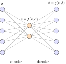
An autoencoder as a two-layer neural network (a schematic): a one-layer encoder compresses into a code vector of smaller dimension, and a one-layer decoder restores a reconstruction of the same dimension as .
Keep in mind what is happening here: in effect a two-layer neural network, a one-layer encoder and a one-layer decoder. The original space is of large dimension, the intermediate one of smaller dimension, and we set this dimension by the number of neurons of the hidden layer. The output layer must by construction have the same dimension as the input one: the reconstruction appears on it, which then has to be compared with the input vector. This is the canonical construction.
Remark (Code vectors at test time). A question: so at the test stage we do not look at the restoring right-hand layer and take the outputs of the middle?
Quite right: we take the new vector representation of the objects at the output of the intermediate hidden layer. Moreover, since linear autoencoders are connected with the principal component method, the matrix is the weights of the encoding layer and the matrix of the decoding one, and in the principal component method they are the same up to transposition: the decoder performs literally the inverse transformation with the same weights. Sometimes the constraint is introduced deliberately, sometimes not; it is a heuristic that may or may not be applied.
How can this construction be generalised? Why must the middle layer be of smaller dimension than the input one; could it not be the other way round? It can, and one of the types will be the sparse autoencoder. It does not compress the original vector representation but, on the contrary, "decompresses" it, but so that the new vector representation contains very many zeros: there may turn out to be very few non-zero coordinates. The point is to find a vector representation in which only some coordinates are non-zero, and this hints that we expect to introduce some interpretation for these coordinates. Each object is now represented not by a dense but by a highly sparse vector of very large dimension, and its coordinates say that some hidden properties are either present in the object or absent. A non-zero -th coordinate corresponds to some hidden property; we have identified a full set of hidden properties, there are more of them than original features, and we can describe each object in terms of what part of these properties it has, and a non-zero value shows the degree to which a hidden property is expressed.
One more generalisation is multilayer autoencoders. It naturally comes to mind: why a two-layer neural network, could the number of layers not be increased? It can, and it is an interesting possibility: to reduce the dimension gradually, and since there are activation functions, a fairly arbitrary nonlinear transformation can be used as the encoder, and then the inverse one, the decoder. Architectures can be one-layer and multilayer, reducing and increasing the dimension.
The sparse autoencoder
We will now go through about seven types of autoencoders.
Definition (Sparse autoencoders (Sparse AE)). Applying or regularisation to the weight vectors , :
Applying regularisation to the code vectors :
Entropy regularisation for the case :
where ; is a parameter close to zero; is the KL divergence.
D. Arpit et al. Why regularized auto-encoders learn sparse representation? 2015.
The point of a sparse autoencoder is to build an intermediate vector description that will have many zeros. For this one can apply, for example, regularisation; this is done in different ways. The first is ordinary LASSO: regularisation, perhaps , they may be used together; this differs little from regression with or regularisation, which we understand well. But there are also rather original approaches. In regression it is usually the coefficients themselves that are regularised, here and , and if these are linear transformations, that makes sense. But if we want sparsity not of the parameters of the encoder and the decoder but of the intermediate representations, the vectors , and the vectors are , then the norm has to be minimised not for and not for but for the intermediate vector representations. So the more reasonable way of regularisation is the second. Note that under the absolute value there is no longer the parameter itself but of ; this is a more complex optimisation problem, a non-smooth one: may be a smooth transformation of , but the absolute value is no longer smooth, and solving it is harder, but there are analogues for it too, subgradient methods.
What else is done? Entropy regularisation. If we are going to zero many components of the vector , let us require that the mean value of the features over the objects be as small as possible. This requirement can be formalised in different ways, in particular through the KL divergence, which requires that the distribution of be close to zero, to a degenerate distribution. Such types of regularisation really can lead to many coordinates of the vectors being either exactly zero or very close to zero, and then we zero them.
Remark (The parameters and). A question: is a distribution?
No, it is simply a small number, close enough to zero, a parameter. is a selectivity parameter: the larger it is, the more components we zero, the higher the selectivity. And for it is the opposite: the smaller it is, the closer to zero the mean value of a feature over all objects will be.
The denoising autoencoder
Definition (The denoising autoencoder (Denoising AE)). Robustness of the code vectors with respect to noise in :
Instead of computing , in the SG method the objects are sampled and noised one at a time: .
Variants of the noise with respect to which robustness is needed:
- , Gaussian noise;
- zeroing components of the vector with probability .
P. Vincent, H. Larochelle, Y. Bengio, P.-A. Manzagol. Extracting and composing robust features with denoising autoencoders. ICML-2008.
A very often used autoencoder is the so-called denoising one. The idea is very simple: the autoencoder should be robust. If instead of the object we take some vectors close to it, they should turn into close codes, and close codes should correspond to close decoded vectors. We add noisy vectors to the criterion: now the vector must not simply be reconstructed but reliably reconstructed from slightly distorted variants. We introduce a probability distribution of given , for example Gaussian noise with variance : we add Gaussian noise to each coordinate of the vector. We feed the noisy to the input instead of the original and require that, although we have spoiled it, still be reconstructed with fairly high accuracy, clearly no higher than the added noise allows. With this requirement we will greatly increase the noise immunity of the whole model.
How is this done? Very simply: in the stochastic gradient method, when we select the object at random, at that moment we add random noise to it. The noise is added only at this iteration; at the next one we take some other object with new noise, and when we again choose this same , we throw a different noise onto it. So the parameters and will be trained without paying attention to the noise; this is a very important property, and it too is a kind of regularisation. We may have redundant degrees of freedom in the parameters and , use a richer family of transformations, but we force them to be noise-immune: the parameters are no longer just anything, they must be such that the reconstruction is reliable despite the noisiness of the original data.
Another variant of noise is zeroing the components of the original vectors. Gaussian noise models errors of physical measurements; its variance is small. And another type of distortion with respect to which one would like a robust reconstruction is when a great disaster happens to individual feature values, but rarely. We will simply zero individual components of the vector with a not very large probability : say, 5 % of the features in the original vector are spoiled, but spoiled badly. One noise model spoils slightly but all the coordinates; the other spoils badly but a small share of the coordinates, simply zeroing them. And despite all these brutal abuses of the original vectors, they should be reconstructed quite well.
The contractive and relational autoencoders
Definition (The contractive autoencoder (Contractive AE)). Robustness of the code vectors with respect to noise in :
where is the norm of the Jacobian matrix of the mapping :
In the case , where is the sigmoid, :
Salah Rifai et al. Contractive auto-encoders: explicit invariance during feature extraction. ICML-2011.
One more variety, applied less often, but also fairly often. The encoder should be a stable mapping, but now in the sense of a contraction mapping: if it is smooth, the partial derivatives should be less than one; the norm of the Jacobian matrix should be less than one or at least as small as possible. So the sum of squares of the partial derivatives is introduced as a regulariser. It is a function of , an additional criterion; in the special case of a neural network autoencoder with sigmoid activation functions it is not at all hard to write it out. It is smooth, it is added to the original functional, and in the stochastic gradient method there is no difficulty at all in adding its partial derivatives with respect to to the gradient.
Definition (The relational autoencoder (Relational AE)). Along with the losses of reconstructing the objects, we minimise the losses of reconstructing the relations between objects:
where is the reconstruction of the object ; is the scalar product (proximity) of a pair of objects; is a threshold function with parameter (if the vectors are not close, it does not matter how far apart they are); is a loss function, for example .
The experiment: the quality of image classification with code vectors improves on the MNIST and CIFAR-10 problems.
Qinxue Meng et al. Relational autoencoder for feature extraction. 2018.
One more idea is the relational autoencoder. Now we want to reconstruct not only the objects themselves but also some relations between them, for example scalar products: if there were some scalar products between the objects and in the original space, we want the reconstructed vectors to preserve them. What for? If is a good reconstruction of , the scalar products will be preserved with some accuracy anyway. The trick is that if we make reconstructions for the sake of passing into the intermediate space and want to use , for example, to compare objects, compute scalar products, look for the nearest ones, if the whole construction is needed in order then to compare the intermediate compressed representations, then it would be good for the scalar products, or those relations between objects that we are going to use later, also to be reconstructed well.
The variational autoencoder
And the last type, which I would like to go through in a little more detail, is the variational autoencoder. I have counted seven main, most often used types already. The variational one differs substantially from all the previous ones in that probability distributions are recovered here: a generative model is built, able to generate new objects similar to the objects of the original sample.
Definition (The variational autoencoder (Variational AE)). Given: a sample of objects .
Find: a model for generating new objects similar to : , a probabilistic encoder with parameter ; , a probabilistic decoder with parameter .
Criterion: the maximum of a lower bound of the log-likelihood:
D. P. Kingma, M. Welling. Auto-encoding Variational Bayes. 2013. C. Doersch. Tutorial on variational autoencoders. 2016.
What is a probabilistic encoder? It is a family of distributions, also with some parameters , that does not simply compute from but is able to generate by some stochastic process: with fixed we can generate , and if we generate a second time, we get some other . What we considered as an encoder before is a special case of a probabilistic encoder with zero variance: there the encoder is a function, and however many times you compute it with and fixed, you get one and the same ; it is a deterministic transformation. A probabilistic encoder is arranged so that, generating many times, we get a new each time. Sometimes this is exactly the effect we are after: for example, if we are going to generate fake objects similar to objects of the real world, the variational autoencoder is a very suitable model for this. We take a particular real-world object from the training sample, generate a representation from it, this generation introduces randomisation into , and then from we reconstruct by the probabilistic decoder. This will be some approximation of the original one, but in this way one can get very many different similar objects. It is a way of generating artificial, fake objects that nevertheless carry the features of real objects. Thanks to what? Thanks to our generating not just some point in the original space close to , which would give an object similar to but unrealistic, but generating it through the hidden representation , which absorbs the whole essence of the object: it is most likely of much smaller dimension, but gathers in itself almost complete information about the object. The realism comes from our having explicitly built the intermediate space in which our real-world objects live.
How is this problem to be posed mathematically? Clearly, two distributions have to be built, a generator of from and a generator of from . Since a probabilistic model is being built, the first thing that comes to mind is the maximum likelihood principle: the likelihood of the reconstruction should be maximal. How is to be written out? Let us introduce the hidden variable : by the formula of conditional probability, is the joint distribution of and , and the integral over of the joint density gives . Then we introduce into this representation: if we write it just like that, there will be a dependence on the parameter and none on , while we need a criterion containing both and . So is introduced absolutely artificially, we divided and multiplied by it, we are entitled to, and we got an equivalent representation of the likelihood functional. Now the clever point: let us use the concavity of the logarithm. The logarithm of an integral is greater than or equal to the integral of the logarithm; if the integral is regarded as the limit of a sum, this is shown in the same way. We bring the logarithm under the integral sign and get a lower bound; it is what we will maximise. This is the essence of the variational approach.
Remark (Why the logarithm can be brought under the integral). A question: could you go over bringing the logarithm under the integral sign again?
Recall the definition of convexity of a function: a function of a convex combination of points, a weighted sum with non-negative weights summing to one. The logarithm is convex upwards, so the logarithm of a convex combination lies higher than the convex combination of the logarithms of these points. Only instead of a sum we have an integral with weights , and this is simply the integral generalisation of the definition of convexity.
Definition (The optimisation problem of the variational autoencoder).
where is the prior distribution, usually .
Reparametrisation of : , .
The stochastic gradient method:
- sample , , ;
- gradient step:
Generating similar objects: , .
The lower bound can be rewritten as the expectation of the logarithm of a probability over the distribution , which resembles the maximum likelihood principle, where the parameter is the parameter of the decoder, minus the KL divergence. But the encoded representation must be generated from a parametric family with an unknown parameter . At first sight a completely crazy construction; we have not solved such problems yet: how do we optimise the parameter if from this parametric family are stochastically generated that figure in a density with the parameter , which also has to be optimised? In fact we will cope with this problem very deftly with a trick called reparametrisation.
The family we are free to set ourselves, as is convenient for us; let us use this freedom. We will not set the family of distributions explicitly, but will compute by some function of and , introducing into this function a random parameter , which for convenience we may take Gaussian. Introducing this parameter is our way of setting a parametric family of distributions. The advantage is that now becomes a parameter inside the differentiable function .
How is the expectation now to be interpreted in the stochastic gradient method? We sample an object of the sample , sample a vector , compute as a function of , and throw out the expectation sign, considering one term. We, as it were, use stochastic gradient twice: the first time we sample an object from the original sample, as we always did, and the second, instead of computing the expectation, we take only one sample of . This is an analogy with how we always sampled in stochastic gradient: originally we optimise a big sum over all objects, and at each step we sample one object and optimise the term over the model parameters. Now we have one more source of randomness, the sampling of , and we agreed to do it by computing a function of , and a random . In a sense, in constructing the probabilistic encoder we have gone back to the ordinary construction of an encoder, a function of and , only we added a random parameter to this function. Having simply computed , we substitute it into the term and take a step over the parameters and for individual terms. The substituted is a smooth function of the parameter , and we can take partial derivatives with respect to ; without the reparametrisation we could not have done this. The regulariser works only on the encoder.
This is the general scheme. For practical application it has to be made concrete: decide on the choice of the prior distribution , this is the Bayesian approach, in it one has to set a prior distribution, and usually a Gaussian with zero expectation is used; decide on the choice of the encoder and on how is generated (usually from a Gaussian distribution); and on the probabilistic decoder, a distribution with parameter . There are many variants of variational autoencoders in which these questions are decided differently, and each time all this will have to be written out; I have given the general scheme from which many special cases are obtained.
Autoencoders for supervised learning
I said that an autoencoder can be used to synthesise a compressed, efficient representation of the original objects, and this representation can be used to solve other problems, for example supervised learning problems. Let us look at this scheme: it is fundamentally important and very often applied.
Definition (Autoencoders for vectorisation and supervised learning). Data: labelled , unlabelled .
Find: , the encoder; , the decoder; , the predictor.
Loss functions are given: , the reconstruction; , the prediction.
Criterion: joint training of the autoencoder and the predictive model (classification, regression or other):
Dor Bank, Noam Koenigstein, Raja Giryes. Autoencoders. 2020.
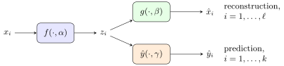
An autoencoder and a predictive model with a common encoder (a schematic): the reconstruction with losses is trained on all objects, the prediction with losses on the labelled ones, and both problems tune the common parameters of the encoder .
We encoded the original , got the intermediate representation , decoded it, got , and in the reconstruction problem must be as close as possible to the original . Next the vectors , as the new vector representations of the objects, are fed to the input of, for example, a classifier that is tuned to the y's, and the task is to require at once both that the reconstruction goes well and that the classification problem on the internal vector representation is also solved well. For this two functionals are combined: to the autoencoder functional responsible for reconstruction, a second functional is added literally as a regulariser, with the loss function you need, responsible for solving the needed problem, be it classification, regression or something else. The main thing is that modified vector representations of the objects are used, new feature descriptions. The encoder and the decoder are built so that the objects get new compressed feature descriptions and so that these descriptions work for solving the needed problem; for all this to happen together, a joint two-criterion problem is solved: the first criterion for reconstruction, the second for solving the needed problem on the new feature description. This scheme has turned out to be very productive and very general, and we will come back to it more than once; the next lecture will be on the synthesis of vector representations of texts and graphs, and there this construction will be generalised very beautifully.
The multilayer autoencoder
Definition (The multilayer autoencoder (Stacked AE)). Layer-by-layer training: , , :
- each pair , is trained on the sample ;
- the decoder is discarded;
- the one-layer are joined into an -layer one.
Fine tuning: the result of layer-by-layer training is used as the initial approximation for BackProp.
Y. Bengio et al. Greedy layer-wise training of deep networks. NIPS 2007.
Multilayer autoencoders exist both for reducing dimension and for increasing it, if sparse ones are built. How are they used? A very simple idea is layer-by-layer training. We build the first autoencoder, an encoder and a decoder, and simply discard the decoder: we have trained a transformation of the original vector into a new one, say of smaller dimension. We use the obtained vector representations as the original ones, build one more autoencoder, compress the dimension still more, and discard the decoder of the second too. Since the second encoder took as input what the first gave as output, they can simply be glued together. In this way the construction can be trained layer by layer, each time throwing out the decoder; the discarded decoders can be glued on in reverse order, or the decoder can be trained anew, as we like. Then the whole construction can be trained once more, fine tuning done; the neural network is already multilayer, and we understand how to further train it by backpropagation so as to improve the result still more.
What is the advantage of multilayer autoencoders? The same idea as in deep neural networks: several nonlinear transformations in a superposition give a very rich family of functions with much richer approximating abilities, a very non-trivial nonlinear transformation of the original objects into a hidden representation. In the middle is a bottleneck through which the original object has to be passed so that inside it there is information about it as complete as possible, and the original object can be reconstructed from it with good quality. Building several such layers, you say: I do not want to know how this bottleneck is arranged, but it must work.
Joint training of several models
Pre-training and transfer learning
Let us return to deep neural networks and recall how a convolutional network for image processing is arranged: there is a very direct analogy with an autoencoder. Several convolutional layers, then a fully connected layer, and, as I said in the last lecture, on the last or the last-but-one layer vector representations of the original images are formed: contracting the size of the picture layer by layer, in the limit we contract it into , but a vector of large dimension sticks out of this pixel. So a convolutional neural network, in our current understanding, is nothing other than an encoder: we have convolved the image into a vector of large dimension, which is still much smaller than the number of pixels; an encoder specially tailored to image processing.
What can we do? A very popular idea is pre-training: such an encoder can be trained on some very large database of images, for example ImageNet, and we get an encoder that can encode an image into a vector, and then do anything at all with this vector, for example solve classification problems. A complete analogy with our scheme: the encoder is built on a gigantic training sample; or rather the other way round, you build this encoder by solving a classification problem. A whole field of ideas arises here. Let us generalise the idea of pre-training neural networks and we get a much more general approach called transfer learning.
Definition (Pre-training, transfer learning). Training a vectorisation model on a sample :
Training the target model on small data :
Sinno Jialin Pan, Qiang Yang. A Survey on Transfer Learning. 2009. J. Yosinski et al. How transferable are features in deep neural networks? 2014.
A convolutional network in fact consists of two parts. The first, convolutional, the most substantial and heavy one, is needed for vectorising images, for synthesising their vector representation. This universal part of the model we can tune once on some very large collection of the ImageNet type, and then use it to solve specific problems on small samples. The base problem allowed us to train the vectoriser , the universal part of the model that assigns to an image a vector preserving all the essential information about the image, and it was trained on a big sample. But we need to solve another problem, not recognising pictures from ImageNet but, for example, learning to tell civilian vehicles from military ones in photographs taken by a drone. The training sample is not very big and certainly not very well labelled: at best several thousand labelled images, a lorry, a tank, an armoured personnel carrier, a car. And this small sample can be used to solve the problem with very high quality, because our image vectoriser is already ready: we trained it on kittens, puppies, little houses and little people, on 15 million images from ImageNet. We fix its parameters , no longer touch them, and use the ready pre-trained vectoriser to solve our problem on a small sample. Solving the problem in this way, in two stages, we get a solution of much higher quality than if we looked for both and at once on our small sample; the problem cannot be solved that way, nothing will come of it. We have used big data to tune the universal part of the model, the vectorisation of images, and the specific part, tailored to our small sample, we trained with the vectoriser fixed. This is somewhat like an encoder and a decoder: we have again sawn the model into two parts, only now they are not symmetric to each other.
Multi-task learning
This idea can be generalised further: there is the concept of multi-task learning, which is in essence slightly modified transfer learning.
Definition (Multi-task learning). is a vectorisation universal for all models; is the specific part of the model for the task .
Simultaneous training of the model on the tasks , :
- Learnability: the quality of solving an individual task improves as the sample size grows.
- Learning to learn: the quality of solving each of the tasks improves as both and the total number of tasks grow.
- Few-shot learning: to solve a new task a small number of examples is enough, even one (one-shot learning).
Yu Zhang, Qiang Yang. A survey on multi-task learning. 2021. M. Crawshaw. Multi-task learning with deep neural networks: a survey. 2020. Y. Wang et al. Generalizing from a few examples: a survey on few-shot learning. 2020.
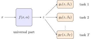
Multi-task learning (a schematic): the universal vectorisation is trained on all tasks at once, and each task has its own specific part with its own parameters . Transfer learning is a special case: is trained on a big task and fixed, and for a new task only its is trained.
Multi-task learning too profits from our building a universal part of the model, for example for vectorising images; although clearly this idea can be generalised and vectorisations built not of images but of some other objects, or in general some hidden vector representations. The main thing is that they must be universal for a large number of tasks of the same type. Tasks of the same type are, for example, all problems of classifying images: human faces, Chinese characters, car number plates. Of the same type because the structure of the input data is one and the same, photographic or scanned images, so the universal convolutional part of the network can be built once for any images. The universal part is trained simultaneously on a large number of tasks. Different tasks are, for example, different samples of images: is the number of a task from the set , and each task has its own training sample, perhaps even its own loss function and its own model, but all the models have a common part, in the case of images a single convolutional network building a vector from an image, and we train it simultaneously on the most diverse image processing tasks. Note that the parameter does not depend on the task ; it is one for all tasks, while the second part of the model is specific, and each task has its own .
Purely conceptually: when we speak in machine learning of learnability, we usually mean that as the size of the training sample grows, the quality of solving the problem improves, in the sense of generalisation ability, in the sense of how the model will then work on test data. A broader concept is learning to learn, or, in effect a synonym, transfer learning: the quality of solving a problem improves not only as the size of the training sample grows but also as the number of tasks we have learned to solve increases, given that all the models have a common universal part, in particular a vectoriser of complexly structured objects. Now we, as it were, learn to learn: we increase the number of tasks we train on, and the quality of solving each individual task grows because they all share a common universal part.
A special case, just to mention it, we will not develop this topic deeply now, is few-shot learning, or one-shot learning: the ability to learn from a very small number of precedents, in the limit even from one. Think about why a person can learn to distinguish different species of birds if shown even one photograph: a secretary bird, a king penguin; it is enough to show one photograph for him to learn to tell king penguins from all others. How can neural networks be endowed with such an ability? It turns out, precisely with such an approach: when you have a reliable image vectoriser, well trained on a large number of different tasks, the training sample for some task can be cut down critically, right down to a single precedent, and one can learn to recognise king penguins from one picture.
Self-supervised learning
One more close idea is a revolutionary thing altogether in the ImageNet story, which showed that, by and large, it was not really necessary to label 15 million images. The idea is called self-supervised learning (not to be confused with semi-supervised).
Definition (Self-supervised learning). The vectorisation model is trained to predict the relative position of pairs of fragments of one image (8 possible positions; a classifier on top of two copies of one CNN).
The advantage: the network learns vector representations of objects without a labelled training sample.
Carl Doersch, Abhinav Gupta, Alexei A. Efros. Unsupervised visual representation learning by context prediction. ICCV 2015.
Instead of labelling a huge number of images, 15 million, by crowdsourcing, let us take the same 15 million photographs and pose a different problem on them, with an artificial training sample that we can generate ourselves. There are many ways, and one of them is to learn to recognise the relative position of pairs of fragments of one image. We take some fragment, a blue square, and around it, shifting slightly, cut out 8 more squares, and form an artificial training sample of pairs of fragments: in this pair the red fragment is at the top right relative to the blue one. There are only 8 possible positions, so this is a problem of classifying pairs of fragments into 8 classes. From each photograph a huge number of such pairs can be cut: for each blue square cut out eight in different positions, and there are also a huge number of ways to cut out these 9 squares. A very cheap way of forming an artificial training sample really does allow big data to be obtained without any involvement of human labour: the classification here is artificially generated. And the miracle is that if a convolutional neural network is built to solve such an artificial classification problem, we get a vectorisation of images in no way worse than a vectorisation trained on the labelled ImageNet. This really is a big miracle and a big breakthrough: much was said about how far ImageNet made possible a breakthrough in training deep neural networks, and in 2015 a new revolution on top of that one: it turns out the 15 million images did not need to be labelled. Who knew; had they known, they would not have spent so much time. But, on the other hand, this made it possible first to learn to build and train convolutional networks, and only several years later did it become clear that it could be done more simply, without making people look for objects in images.
Self-supervised learning is a very serious idea, and it was further generalised and transformed for training language models, for text processing and for much else. If you have complexly structured objects, images, signals, graphs, then, using their internal structure, you can synthesise artificial training samples and build very high-quality vectorisations on them. And if you have managed to make a vectorisation of a complexly arranged object that allows a non-trivial problem to be solved, and predicting the neighbourhood of fragments is a very non-trivial, very hard problem, then there will be success in solving a big heap of problems that will use these vectorisations; recall transfer learning.
I am telling all this without much depth, broadly, as it were, but it is important to see the commonality: convolutional networks for image processing, autoencoders, pre-training, transfer learning are all strung on one common idea, which can be briefly formulated thus: we train several models at once. Let us go further with this thought in mind.
Distillation and surrogate modelling
Definition (Model distillation, or surrogate modelling). Training a complex model , "long and expensive":
Training a simple model , possibly on other data:
Examples of problems:
- replacing a complex model (climate, aerodynamics, etc.) that is computed on a supercomputer for months by a "light" approximating surrogate model;
- replacing a complex neural network that is trained for weeks on big data by a "light" approximating neural network with a minimised number of neurons and connections.
One more special case is called distillation, and a little earlier it was called surrogate modelling. Suppose we have learned to build some very complex model, for example trained a deep convolutional network on ImageNet, on 15 million images, and spent an incredible computational resource, a lot of money, a lot of electricity. The model is insanely complex: for example, even trained, it cannot be squeezed into a smartphone; there are not enough resources simply to compute this network on a given image. There are many such examples, and there are examples from industry that arose much earlier than convolutional networks: computations on supercomputers, climate models, models of aerodynamics, for example of an aircraft wing, which take months and cost huge money, but one wants to use such models many times without resorting to supercomputer computations. This is what is called surrogate modelling: one wants to approximate a very complex multi-parameter model by a model with orders of magnitude fewer parameters, so that the accuracy does not suffer much. We are ready to sacrifice half a per cent, a tenth of a per cent of accuracy, but reduce the number of parameters tens or hundreds of times. It turns out that such things really do work: super-complex models have redundancy; we simply do not yet know how to build them simple from the start. In recent years, in connection with neural networks, this has come to be called distillation.
How is a surrogate model trained? If the original model was trained by some loss function and by the teacher's information, there were y's for our x's, then the surrogate model can be trained by replacing the y's with what the complex model produces: now it is, for us, the reality that we model. Why not substitute the original y's? Because the complex model allows a much larger training sample to be made: one can generate a heap of new x's and use not the true y's but the model's answers on the new training sample, and it may be much larger than the original. On expensive computational resources we built a model, computed it on a new training sample, and on it we build a second model, much simpler, which will fit into a smartphone.
Learning using privileged information
There is one more very close concept, which at the level of the formulation of the problem practically coincides with distillation, although at first sight it concerns a quite different situation: learning using privileged information.
Problem formulations in terms of data (slide): the training part (top) and the test part (bottom); are the features, the answers, the privileged information, available only in training. V. Vapnik, A. Vashist. A new learning paradigm: Learning Using Privileged Information. Neural Networks, 2009.
There are six pictures here; you already know the left ones. In supervised learning there is an "objects–features" matrix, the rows are objects, the columns features, on the training sample the correct answers are known, and on the test there are no answers; those are what we want to obtain (red in the picture). In unsupervised learning there are no answers even in training; you solve a clustering problem on the x's. Semi-supervised learning differs in that a small piece of the training sample is labelled. And privileged learning is when on the training sample you know some additional information about your objects and can use it for modelling, but the trick is that this information will not be there at test time.
Example (Examples of problems with privileged information).
- is the primary (1D) structure of a protein; the tertiary (3D) structure of the protein; a hierarchical classification of the protein's functions.
- is the prehistory of a time series; information about the future behaviour of the series; the forecast of the next point of the series.
- is a text document; highlighted keywords or phrases; the category of the document.
- is a (query, document) pair; keywords or phrases highlighted by an assessor; a relevance score.
An example is the classification, or categorisation, of text documents. You form a training sample with the help of assessors: an assessor must assign a document to some categories, the classical formulation of the categorisation problem. But suppose you ask the assessor, a specialist in the subject area or a linguist, to give additional information: to highlight in the text the keywords or phrases thanks to which he decided to assign the document to precisely this category. is formed, additional information, finer and more substantive, which allows the categorisation problem to be solved much better. But the trick is that this kind and knowledgeable assessor will not be there when you are solving the categorisation problem in production on new incoming texts: everything there has to be done automatically, and it will not be possible to ask a person to make ; at test time the privileged information is absent. But it can help build a more substantive, better model: the assessor shows how the category of a document is connected with some of its properties, for example with keywords.
Definition (The problem of learning using privileged information). Separate training of the student model and the teacher model :
The student model is trained to be no worse than the teacher model :
Joint training of the student model and the teacher model :
D. Lopez-Paz, L. Bottou, B. Schölkopf, V. Vapnik. Unifying distillation and privileged information. 2016.
The scheme of solution is this. First the models can be trained separately. The teacher model differs in having access to the privileged information. If trained separately, the student model, which has no access to the privileged information, is your classical situation. But let us connect the two training procedures and force the student model to work the same way as the teacher, including repeating the teacher model's errors. It is assumed that the teacher model, on the basis of the privileged information, will work better; it will have higher quality. Having trained the teacher model, you can then train the student model from it, or you can train them jointly. This situation very much resembles transfer learning and distillation: you train several models and can train the weaker model either on the original data or on the answers of the stronger model. The formulations of the problems for privileged information and for distillation come out very similar.
Generative adversarial networks (GAN)
The last story of today, which of course deserves a lecture of its own, but now I will explain the main idea in a couple of slides, is generative adversarial networks, which replaced variational autoencoders. The main point of the variational autoencoder is to generate fake objects very similar to real-world objects. But if one tries to generate with it, for example, realistic photographic images, nothing will come of it: autoencoders still lack something for generating high-quality artificial images very similar to real ones, for example generating faces that are not the faces of real people, but a person looks and sees no artefacts saying that the face is not genuine. To solve such a problem with high quality, one again has to build two models at once that will train each other; this is probably the central idea of the third part of the lecture. But here the simultaneous training of two models is arranged much more cunningly: they play a zero-sum game against each other. The two models are the generator and the discriminator. The generator learns to produce fake objects similar to the real-world objects from the training sample, and the discriminator solves a two-class classification problem: it has two types of objects, real-world objects from the training sample and objects that the generator has just generated. The discriminator wants to learn to tell them apart as accurately as possible, and the generator, on the contrary, learns to deceive the discriminator.
Definition (The formulation of the GAN problem). Given: a sample of objects .
Find: a probabilistic generative model ; a probabilistic discriminative model .
Criterion: the maximum of the log-likelihood for the discriminative model :
training the generative model on random noise :
Ian Goodfellow et al. Generative Adversarial Nets. 2014.
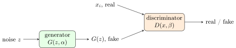
A generative adversarial network (a schematic): the generator turns a random vector into an object, the discriminator learns to tell the real objects of the sample from the generated ones, and the generator learns to deceive it.
Let us begin with the probabilistic model for the discriminator. It solves a two-class classification problem: the posterior probability of the class means that the image is genuine, not fake; of the class , that it is fake. We train the discriminator by the maximum likelihood principle; what is unusual here is that the objects of the first class are real-world objects from the original training sample, and the objects of the second class have just been generated by the generative model . How does it work? At the input it takes some random vector, a hidden representation , an analogue of what an autoencoder builds, only we generate it purely at random, and it must learn to generate a realistic object from it. The generator has its own parameter vector , the discriminator its own, , and they are trained in turn. Training the discriminator, we maximise the likelihood criterion: we want to train the model of the posterior probability of the class "fake or not fake" as well as possible. And the generator plays against the discriminator: it, on the contrary, minimises the same functional. We get a minimax formulation of the problem, as befits game theory: two players play a zero-sum game against each other. maximises the functional over its parameter , minimises the same functional over its parameter ; since the first term does not depend on , the formulation for is a little simpler. The two formulations of the problem, mixed, take gradient steps by the stochastic gradient method, and two models, the discriminator and the generator, are trained jointly.
Remark (Examples of GANs for synthesising images and video).
- Applying an artist's style to photographs. Chuan Li, Michael Wand. Precomputed Real-Time Texture Synthesis with Markovian Generative Adversarial Networks. 2016.
- Recovering a three-dimensional model of a face from one photograph. Xiaoxing Zeng, Xiaojiang Peng, Yu Qiao. DF2Net: A Dense Fine Finer Network for Detailed 3D Face Reconstruction. ICCV-2019.
- Transferring a dancer's movements to a person from one photograph of them. Caroline Chan, Shiry Ginosar, Tinghui Zhou, Alexei A. Efros. Everybody Dance Now. ICCV-2019.
There is a huge amount of literature, good surveys and research on GANs: this model has become very popular and is used in a huge number of applications. I will mention three papers. The first, one of the first on images, from 2016: people learned to use generative adversarial models to apply an artist's style to photographs. If there are many paintings by one artist, one can separate the texture of the style from the content of the image and learn to apply this style to new images: in the style of a marine painter one can make an artistic interpretation of a photograph. Another application already has to do with one-shot learning: how to recover a three-dimensional model of a face from one photograph. There is a training sample of images photographed from different angles; it is used as self-supervised, but it is solved jointly with a problem that allows a three-dimensional model of a person to be built from one photograph of him; the industrial application is clear, for example making three-dimensional models of actors for films or of cartoon characters more efficiently. And one more application from a 2019 computer vision conference: a professional dancer's dance is filmed, then one photograph of a person is taken, even against some background, and we make him dance the whole dance. Also one-shot learning and combining two problems in one criterion.
Conclusions
Remark (Summary). When several models are trained simultaneously:
- autoencoders: the encoder and the decoder;
- autoencoders for predictive modelling;
- multi-task learning;
- learning using privileged information (LUPI);
- adversarial networks (GAN) for generating fake objects.
When several models are trained sequentially:
- transfer learning;
- pre-training of deep networks for vectorising objects;
- self-supervised learning;
- distillation and surrogate modelling.
Unsupervised learning is used more and more often to optimise part of a model on big data.
As a summary I have recapped everything told today by this discriminating feature: in some situations several models are trained simultaneously, autoencoders, multi-task learning, learning using privileged information, GAN; in others sequentially: transfer learning, pre-training in deep networks, self-supervised learning, when we first train a vectoriser on an artificial problem of classifying the relative position of fragments, and surrogate modelling. The common idea running through all these problems is the joint training of several models, but they may be trained in parallel or sequentially.
No comments yet
Be the first to share your thoughts.