August 30, 2026 · Lecture · LibreTimes
Machine Learning 1. Lecture 13. Clustering and Semi-Supervised Learning
Contents
- What this lecture is about
- The problems of clustering and semi-supervised learning
- The clustering problem
- The ill-posedness of the clustering problem
- The aims of clustering
- Types of cluster structures
- Sensitivity to the choice of metric
- The semi-supervised learning problem
- SSL reduces neither to classification nor to clustering
- Criteria of clustering quality
- The k-means method
- The formulation of the problem and Lloyd's algorithm
- k-means for semi-supervised learning
- k-means as a simplification of the EM algorithm
- Unfortunate initial approximations
- The DBSCAN algorithm
- Hierarchical clustering
- The Lance–Williams algorithm
- The Lance–Williams algorithm for semi-supervised learning
- Special cases of the Lance–Williams formula
- The dendrogram
- Monotonicity, contraction and dilation
- Recommendations and conclusions
- Semi-supervised learning based on classification
- Self-training
- Co-training
- Co-learning
- The general optimisation approach
- The transductive SVM
- Expectation regularisation (XR)
- Conclusions
- Seminar
What this lecture is about
The topic we will discuss today we began a little in the last lecture, when we talked about separating a mixture of distributions: I said then that this is clustering, and promised to continue the topic. Today will be about unsupervised learning, and we will also touch on the topic of semi-supervised learning: there is a teacher, but not much of one. The lecture is packed; let us take everything in order.
The problems of clustering and semi-supervised learning
The clustering problem
Let us begin with the notation. As usual, there is a training sample. All semester we have solved classification and regression problems in which each was assigned a . Today it will not be so, or "half not so": in semi-supervised learning some objects will after all be assigned a . And the clustering problem is this: from information about the objects, we must split them into compact clumps of points, clusters. They are deliberately called clusters rather than classes, as usual. And usually even the number of clusters is not known in advance.
Definition (The informal formulation of the clustering problem). Given:
- , the space of objects;
- , the training sample;
- , a distance function between objects.
Find:
- , the set of clusters,
- , the clustering algorithm,
such that
- each cluster consists of close objects;
- objects of different clusters are substantially different.
This is an unsupervised learning problem. The criterion?
We have to build a clustering algorithm, a mapping from the set into the set of clusters ; formally it is the same as a classifier. But what the clusters are is not said in advance; we must determine that ourselves from the objects. We are given only a distance function between objects and the hypothesis that each cluster consists of close objects, while objects of different clusters are substantially different. These are two principles that can be formalised however you like: there is no single convention, and many criteria can be invented. And there are also many heuristic methods, where there is a clustering algorithm in itself, but what it optimises is unclear, and one should not even ask that question.
The ill-posedness of the clustering problem
Definition (The ill-posedness of the clustering problem). The solution of the clustering problem is fundamentally ambiguous:
- there is no exact formulation of the clustering problem;
- there are many criteria of clustering quality;
- there are many heuristic clustering methods;
- the number of clusters is, as a rule, not known in advance;
- the result of clustering depends strongly on the metric , whose choice is also a heuristic.
Moreover, we will now see on examples that the result of clustering may depend on the distance function. And its choice is also a heuristic, and it depends on the whim of the researcher, on the whim of the client, on some knowledge of the subject area that may be inaccurate, incomplete, partial. And here is one more picture: how many clusters are there here? One can say two, one can say four, one can say six, and we will all be right.
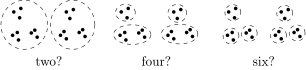
How many clusters are there here? The same points can reasonably be split into two, four or six clusters.
The problem is ill-posed, but one still wants to solve it.
The aims of clustering
Why does one want to solve it? There may even be many aims.
Definition (The aims of clustering).
- To simplify further processing of the data: split the sample into subsamples of similar objects and then work with them on the "divide and rule" principle (in problems of classification, regression, forecasting).
- To reduce the amount of stored data, leaving one representative of each cluster; to get the most representative subsample.
- To single out atypical objects that do not fit any of the clusters (anomaly detection, one-class classification).
- To build a hierarchy of the set of objects; an example is C. Linnaeus's classification of animals and plants (problems of taxonomy, of hierarchical clustering).
The first is to simplify further processing of the data. If there are compact clumps of points, clusters, among the data, then each cluster can, as it were, be replaced by one point, one typical representative, and we can say: everything nearby is almost the same. Sometimes this succeeds, and in this way we simplify the problem. One can even reduce the amount of stored data, keeping only typical representatives, the standards of each cluster. Or perhaps, on the contrary, the problem is to find objects that are like nothing else; this is called anomaly detection, or outlier detection; clustering can be used for this too.
And finally, one can pose the problem of building a hierarchy of the set of objects: first single out large clusters and thereby understand the structure of the space of objects, then begin to split each cluster into smaller ones, then the smaller into still smaller ones and so on. This is called hierarchical clustering; we will look at such approaches today too. An example is Carl Linnaeus's classification of animals, plants and minerals; this is also called the problem of taxonomy. Before us is a huge number of objects, species of animals and plants, and one wants to group them somehow by some features. Carl Linnaeus, long before the computer era, was in fact doing clustering: he literally wrote cards on which he described the features of species, made a huge card index, and then compared them; in essence, he estimated the distances between his cards describing species. That is how he got levels of clustering, and now biologists keep introducing still more new levels. It is an attempt to order, to bring some structure into a large, complexly arranged finite set of objects. So I hope I have convinced you that, despite the ill-posedness of the problem, it has to be solved.
Types of cluster structures
When people talk about clustering, the first thing that comes to mind is a structure like this: three round clusters. But that is not always so.
Types of cluster structures (slide): clusters with centres; intra-cluster distances on the whole smaller than inter-cluster ones; ribbon clusters.
It may be that there is no such clear division between clusters. Or here, for example, are ribbon clusters: to say that distances within a cluster are smaller than between clusters would simply be wrong, yet with our eyes we see two clusters here. They need not be ball-shaped clumps of points; the shape may be anything at all.
Types of cluster structures (slide): bridges between clusters; a sparse background of atypical objects; overlapping clusters.
Or we may want to use some graph algorithm, and here is a counterexample: a graph algorithm will not work here, because there are bridges between the clusters. Or here is a sparse background: there are three clusters, and there is a background, and, as I said, we may even deliberately chase the background objects, the aim may be to single them out, or perhaps they will hinder us in doing the clustering. And finally, overlapping clusters. You already guess that such clusters are just the thing to separate as a mixture of probability distributions by the EM algorithm, what we looked at in the last lecture. Simple approaches, like "let us single out for each object the ones nearest to it", clearly will not work here, while separating a mixture of distributions, when we look at the whole sample at once and can see that there are two overlapping clusters here, may work.
Types of cluster structures (slide): there may be no clusters at all; and these are not clusters at all, and in practice this does not occur.
And here is a situation that often arises in practice: there are no clusters at all. A client may come and say: "Do me a clustering of the customer base." He has a million customer points there, and you, however you twist it, in whatever feature space, whatever metric you introduce, keep seeing this picture: there is a clump, the bulk of the customers form a certain single typical behaviour, and the farther from this typical behaviour, the rarer the customers. It is all one, a unimodal distribution.
And the last picture is a purely geometric problem. Intuitively we see two clusters here, an arc and a grid. Of course this does not happen in practice, but such counterexamples can be invented to catch clustering algorithms working incorrectly: clearly any algorithms based on distances between points will not work in this problem.
Remark (The type of cluster structure).
- Each clustering method has its own limitations and singles out clusters of only some types.
- The notion of a "type of cluster structure" depends on the method and also has no formal definition.
Each method is aimed more at some things and less at others. And the very notion of cluster structure is not formalised: it depends on the method and perhaps on the optimisation criterion; we will now see what criteria can be introduced here too.
Sensitivity to the choice of metric
One more reason for the ill-posedness of the problem is the sensitivity of clustering to the choice of metric. I took this picture from some old textbook, still from Soviet times, that told about the clustering problem. A group of students was taken, and points were plotted in the axes of two coordinates, weight in kilograms and height in centimetres, and it was seen that the clusters are interpretable: there are female students and there are male students. Then the scale was reduced on the horizontal axis. The metric changed: it is the same one, the Euclidean metric on the two-dimensional plane, only one of the features began to be taken into account with a smaller weight. And what did we see? A completely different interpretation: a different cluster stood out: there are tall boys and everyone else.
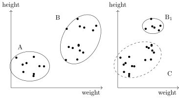
The result depends on the normalisation of the features (a schematic). Left: in the "weight–height" axes the clusters A, the female students, and B, the male students, stand out. Right: the same points after the weight axis is compressed twofold; now it is more natural to single out the cluster B, the tall students, and C, everyone else.
So everything depends on the metric. But we will now assume that a reasonable, correct metric has been given to us by someone from above, we do not doubt it and work with what there is. If there is a different metric, there will be a different clustering result.
The semi-supervised learning problem
Now a little about the second formulation of the problem. I will often run them in parallel, because many methods are very easily adapted to this second formulation. We call it semi-supervised learning, SSL. The point is that we may have very many unlabelled objects, but on a small part of them we have still managed to get labels of classes or clusters; here it is even unclear what to call them properly. Probably it is still closer to the classification problem, because the set of classes is specified here, a finite set, and some subset of objects , small though it may be, is labelled.
Definition (The formulation of the semi-supervised learning problem (SSL)). Given: a set of objects , a set of classes ;
- , labelled objects (labeled data) with labels ;
- , unlabelled objects (unlabeled data).
Find (two variants of the formulation):
- a classification algorithm , the problem of semi-supervised learning;
- the labels of the objects , the problem of transductive learning.
Typical applications: classification and cataloguing of texts, images, etc.
Here several variants of the formulation are distinguished, a fine terminological difference. Semi-supervised learning is when we build an algorithm that, for an arbitrary object , gives us its membership in a class. There is another formulation, which is called transductive learning. Transduction is neither induction nor deduction. Deduction is from the general to the particular, induction from the particular to the general. By the way, all of machine learning is sometimes called empirical induction: from a sample we build some general mapping, recover a function from points. But here it is neither the one nor the other; here it is transduction, from the particular to the particular: we know in advance all the objects on which we lack labels, and must synthesise these labels. Knowing all the objects in advance, the whole unlabelled sample, immediately immerses us in the specifics of the clustering problem, and information about the whole unlabelled sample may help to do either classification or clustering. The specificity of transduction is that we have agreed in advance: there will be no more new objects; only these unlabelled objects have to be labelled.
Typical applications are categorising texts, images, music. Here we have millions of music tracks, and we want to classify them by genre. We seat a number of people who understand music, with a musical education; they sit and label, it is long and expensive, but they have labelled some part of the sample, not millions, of course, a couple of thousand, say. We have both labelled and unlabelled objects, and it would be a sin not to use this situation to combine the solution of the classification problem on the labelled data and of clustering on the unlabelled data.
SSL reduces neither to classification nor to clustering
The first example. Suppose we have two Gaussian distributions with the same variance. Clearly the separating surface between them, according to Bayesian classification theory, which we studied last time, will be linear. But if we have been given only a few labelled objects from each distribution, five each, they will not be enough to understand that these are two spherical Gaussians. And here is the result: a quadratic separating surface that has gone God knows where. But if you had been given the unlabelled objects in advance as well, you would have recovered the mixture of distributions, understood that these are two Gaussians, built a Bayes classifier from them and got what is needed.
The second example is a textbook one; the problem is called "two moons", or "two bananas"; it is called differently. Two clusters, and it seems clear by eye how they should be separated. And now we are given a training sample: one object of one class and one object of the other, and solve it however you like.
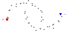
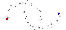
The "two moons" problem (a schematic): the grey points are unlabelled objects, the square and the triangle are the only labelled objects of the two classes. Classification methods will not separate the moons from two objects, while the cluster structure of the unlabelled data sees them at once.
Clearly no nearest neighbour methods, separating surfaces or decision trees will separate these two bananas for us in the conditions of a super-small sample. But if we solve this problem as clustering, we will of course see these two bananas, then see one labelled point in each of them, and this information will be enough for us to label all the others correctly.
The opposite situation: SSL does not reduce to clustering either. Why? Because the teacher who has given us labels, on rare objects but labels all the same, is more important to us than the cluster structure of the data. Here comes the teacher and says: this is one class, and this point from the lower banana is the same class, and that is that. We will be forced to cut the lower banana into two halves, because we trust the teacher more than our own eyes, the metric, the cluster structure and so on.
Remark (SSL reduces neither to classification nor to clustering).
- Example 1: the class densities recovered from the labelled data and the densities recovered from the full data give different separating surfaces.
- Example 2: classification methods do not take into account the cluster structure of the unlabelled data.
- Example 3: clustering methods do not take into account the priority of the labelling over the cluster structure.
Such is the specificity of the problem: such a cunning intermediate formulation between classification and clustering. We will run these two formulations side by side, because it is very convenient, having talked about some clustering algorithm, to say: and now, by correcting one line of code, we will adapt it to solve the semi-supervised learning problem. And in the last part of the lecture we will do the opposite: we will consider classification algorithms and adapt them to semi-supervised learning, and there much greater difficulties await us. That was a spoiler.
Criteria of clustering quality
Let us discuss one more general question: how is the quality of clustering to be measured, and can clustering be posed as an optimisation problem at all? Generally speaking, it can, but in different ways.
Definition (The quality of clustering in a metric space). Let only the pairwise distances between objects be known; is the clustering of the object .
The mean intra-cluster distance:
The mean inter-cluster distance:
The ratio of the pair of functionals: .
The most commonly used way to measure quality is to compute the mean intra-cluster distance, over all pairs of objects lying in one cluster, and the mean inter-cluster distance, over all pairs of objects that lie in different clusters. We get two metrics, and they can be aggregated somehow: for example, take the ratio, one can take the difference, or something else. And what is the drawback? That one has to go over pairs of objects; that is quadratic complexity in the number of objects.
Definition (The quality of clustering in a linear vector space). Let the objects be given by vectors .
The sum of the mean intra-cluster distances:
where is the cluster , the centre of mass of the cluster .
The sum of the inter-cluster distances:
The ratio of the pair of functionals: .
Can it be done faster? It can. If the objects are given by feature vectors, we can be cunning and say: we have cluster centres; the clustering method does not simply single out some set of objects but indicates in it a typical representative, a centre. And then the intra-cluster distance is the distance to the centre, and the inter-cluster distance the distance between centres, and that is all. Computing these distances, both intra-cluster and inter-cluster, becomes of the order of the sample size, that is, they can be estimated faster. These two criteria too have to be aggregated somehow: either look at both separately, or take their quotient, or their difference, or something else.
The silhouette coefficient
And here are a few non-trivial ways of measuring the quality of clustering. The first is rather old; it is needed to understand how the clusters are arranged at all and how well each cluster has formed. It is called the silhouette coefficient.
Definition (The silhouette coefficient (Rousseeuw, 1987)). The distribution of clustering quality over objects and clusters.
The mean distance to the objects of one's own cluster:
The minimal mean distance to another cluster:
The silhouette coefficient of an object:
What is the point? Let us take each point in each cluster and estimate how large the mean distance to the objects of its own cluster is. Then let us measure the mean distance to the objects of each other cluster and take the minimum over all other clusters. And we make a relative measure. We expect that the distances to the objects of one's own cluster, the small , will be less than the big , that is, intra-cluster distances smaller than inter-cluster ones. The silhouettes of all objects are drawn in one picture, cluster after cluster. On the slide four clusters have formed, A, B, C, D, and they are all very good, because the silhouettes of all objects are greater than zero: one's own objects are on average closer than the nearest other cluster.
The technique is a visual one and, although old, is still recommended for use. If you are solving a clustering problem, it is very good to look at how well the clusters have formed. If you have a cluster whose silhouettes are negative, something is wrong there: perhaps you did not guess the number of clusters, and it has to be merged with some other cluster. Then you decide about correcting the clustering.
Precision and recall compared with a reference
One more approach. There are situations where we do a clustering and manually label the objects by classes on part of the sample, and want the algorithm to reach a quality as if we did know the class labels. That is, we do a labelling deliberately, simply to check whether our clustering algorithm works correctly. No training takes place on the labelled objects; they are only for validation.
Definition (The BCubed measures of precision and recall of a clustering). is the reference classification of the objects, . The problem: the cardinalities and may not coincide.
- is the cluster of the object ;
- is the reference class of the object .
So we have a reference classification of the objects, and the number of clusters may even not coincide with the number of classes. What do we do? We say: is the cluster of the -th object, all the objects of the sample that the clustering algorithm assigned to the same cluster as ; and are the objects of the same class in the reference labelling. Now for each point we have two finite sets of objects, and we have to understand how well they coincide with each other. How to measure it we know: we measure precision and recall. But since precision and recall are measured relative to each object, we make the mean precision and the mean recall, aggregating them over all objects.
How to construct such functionals we will not go into further; what has been said is enough. So we have discussed the formulation of the clustering problem, the formulation of the semi-supervised problem, when part of the objects is labelled, and some criteria for measuring the quality of clustering, and therefore some considerations on how to turn clustering into an optimisation problem. We move on to the methods.
The k-means method
The formulation of the problem and Lloyd's algorithm
Let us use these considerations to understand how what is probably the most popular, well-known and simplest clustering method works, which is called k-means. It is an optimisation algorithm that minimises the sum of squares of intra-cluster distances.
Definition (The k-means method: the formulation of the problem). Given: , a training sample, .
Find:
- the cluster centres, the parameters , ;
- which cluster each object belongs to: .
Criterion: the minimum of the sum of squares of intra-cluster distances
The metric is, as a rule, Euclidean (but may be another one):
Here is the number of the cluster to which the object will be assigned, and the problem is posed like this: the distances from the objects to the centres of their clusters must be minimal. The distance is defined as Euclidean. I note: if you should want to replace the Euclidean distance by some other one, you will get, generally speaking, a different algorithm. Lloyd's algorithm is an optimisation method for solving precisely this problem with Euclidean distances in : both the objects themselves and the cluster centres are vectors from .
Definition (Lloyd's algorithm). Input: , . Output: the cluster centres , .
- the initial approximation of the centres, for all ;
- repeat
- assign each to the nearest centre: , ;
- compute the new positions of the centres: , ;
- until the stop changing.
We solve this problem insanely simply. First we take some initial approximation of the centres. We assign each object to the nearest centre by the obvious formula: we have the centres, so we can assign each object to the nearest centre; that is . And then for each cluster we compute the centre of mass, a physical analogy: we simply average our over all the points that are in the cluster. That is it, we have a new approximation of the centres, and we can repeat this iterative process until convergence sets in.
k-means for semi-supervised learning
You should, of course, see what this resembles: it resembles the EM algorithm. We will now consider these two algorithms together, but first, I did promise semi-supervised learning. I will show that Lloyd's algorithm can be adapted for SSL by correcting one line of code.
Definition (The k-means method for semi-supervised learning). A modification of Lloyd's algorithm when there are labelled objects .
Input: , . Output: the cluster centres , .
- the initial approximation of the centres, for all ;
- repeat
- assign each to the nearest centre: , ;
- compute the new positions of the centres: , ;
- until the stop changing.
Suppose we have labelled objects, few of them, the first objects. What has to be done to take this labelling into account in the algorithm? Almost nothing: at the step of assigning to the nearest centre we must take only the unlabelled objects, from to . That is all, no other modifications. The labelled objects already have their class labels, and so the clusters will form around them: we take them into account at the stage of computing the new cluster centres.
k-means as a simplification of the EM algorithm
Now the analogy proper. Let us recall the beginning of the last lecture, when we talked about separating a mixture of distributions with the EM algorithm. If we have the assumption that the mixture components are Gaussian, and with diagonal covariance matrices at that, then the algorithm is written out very simply.
Definition (The EM algorithm for separating a mixture of Gaussians (GMM, Gaussian Mixture Model)). The EM algorithm is likelihood maximisation for separating a mixture of Gaussians.
- the initial approximation , , for all ;
- repeat
- E-step: assign each to the nearest centres:
- M-step: compute the new positions of the centres:
- until the stop changing.
There were two steps there. The E-step computes the posterior probabilities of the clusters for each point, the probability of having been generated by each of the clusters. This is merely Bayes' formula: knowing the cluster centres, we can compute these . This is soft clustering: we have, as it were, smeared each object over all the clusters. But we can assign the object to the cluster for which this probability is maximal, in effect, here it is, the Bayes optimal decision rule, that is, compute , hard clustering.
And the second, the M-step: knowing the degree of membership of each object in each cluster, , what do we compute? In essence we weight all the objects and compute the mean over the objects; that is the centre of the cluster. Here I have also written this out by features, being the indices of the features: such a not vectorial but coordinatewise notation of how we compute the centres of each cluster. The same for the variances, and the variances are in effect the radii of the clusters; we can estimate them here too, and for each feature separately. What does this mean? That our cluster is of elliptical shape: we generalise a little and say that the features may be measured on different scales, so we will not necessarily find spherical clusters; determining clusters of elliptical shape is no harder at all. And are the weights, the estimates of the prior probabilities of the clusters: roughly speaking, the share of the points of the sample that is in this cluster; also by the EM algorithm formula.
So look how similar this is to the k-means method. Let us flip back once more to Lloyd's algorithm: we are doing essentially the same thing. Assigning each object to the nearest cluster is hard clustering, as if at the E-step of the EM algorithm. The new position of the centres is as if the M-step, only no estimation of variances takes place for us: we assumed that they are all the same over all features, that is, the Gaussians are spherical and of the same shape. It turns out that Lloyd's algorithm, although it optimises a quadratic functional, the sum of squares of intra-cluster distances, can also be regarded as a hard coarsening of the EM algorithm for separating a mixture of spherical Gaussians. Literally: we will not estimate probabilities but estimate the degrees of membership of objects in clusters hard right away; we will not estimate the sigmas but estimate only the expectations; and we will give the clusters equal weights. Such a simplification of the EM algorithm gives k-means. Such is the interesting insight.
Remark (Comparing the EM algorithm for GMM and the k-means method). The main differences of GMM-EM and k-means:
- GMM-EM: soft clustering, ; k-means: hard clustering, ;
- GMM-EM: the clusters are elliptical, tunable; k-means: the clusters are spherical, not tunable.
Hybrids (a simplification of GMM-EM, a complication of k-means):
- GMM-EM with hard clustering at the E-step;
- GMM-EM without tuning the variances (spherical Gaussians).
Drawbacks of k-means:
- sensitivity to the choice of the initial approximation;
- slow convergence.
Once more: a Gaussian mixture is soft clustering, we estimate degrees of membership; k-means is hard clustering, each object belongs to exactly one cluster. In the mixture the clusters are elliptical, and tunable at that, while in k-means the clusters are spherical and not tunable, meaning the tuning of variances. Understanding that these come out as two methods from one family, one can arrange hybrids. One can, for example, do a Gaussian mixture but with hard clustering at the E-step: compute as degenerate discrete distributions on the set of clusters and substitute them into the formulas of the M-step. This can be done, but it will not be better, it will only be worse: hardness worsens convergence. One can also say this: the EM algorithm is an advanced variant of the k-means method with improved convergence.
The drawbacks of k-means, and partly of the EM algorithm: it is a method very sensitive to the choice of the initial approximation; I will show examples now, I promised them back in the last lecture, by the way. And convergence is not fast, especially when there are very many points and a big sample has to be clustered. In the literature one can find original papers about a fast stochastic variant of the k-means method, which is recommended when there are many data.
Unfortunate initial approximations
Examples. A problem with three clusters was taken, and a failure happened: two points were initialised in one big cluster, and the third in the third cluster. And it turned out that the big red cluster did not form, it split, while a small cluster that was originally to the side went into another cluster, because of an unfortunate initial approximation. And here is another situation: the initial approximations all fell into one cluster, and the cluster structure, instead of forming three vertical clusters, was cut the other way, horizontally, and we cannot get away from this solution anywhere. Clearly these are specially selected counterexamples, but such situations can still arise in practice.
How to fight them? The answer is multistart. You choose initial approximations some twenty times, start the clustering algorithm from each, and then compare the clusterings obtained by those very criteria I showed, the ratio of intra-cluster and inter-cluster distances.
And here is a situation where nothing will help: however you twist it, you will not separate these little rings. The k-means method and even the EM algorithm with Gaussian components will be able to do nothing here. The only way out is to build not two clusters but, say, 20 or 40, so that small spheres cover these big, clearly non-spherical structures. There is no other way; there are other algorithms that cope with this; about them later.
Remark (Why k-means cuts clusters "the wrong way"). A question: k-means, by minimising distances, seems to gather everything into a cloud; how, then, do stripes come about, why did horizontal clusters come out instead of vertical ones?
In the last lecture I showed how the iterations of the EM algorithm are arranged: first we coloured all the points in the colours of the clusters, then from the coloured points the centres shifted, and little by little, in 20 iterations, they took an almost ideal position. What hinders k-means? A large gap between the clusters hinders it. If the clusters were not at such a large distance from each other, all would be well: the centres would gradually move to their places. But this did not happen, for a paradoxical reason: with large distances between clusters, the k-means method has a hard time. If the initial approximation for a centre turned out to be in another cluster, while the right cluster is far away, then no points of the right cluster are found nearest to this centre, and the centre cannot move in its direction: points from the right cluster simply do not get into its cluster in any way. This is a drawback of the iterative process of the k-means method itself.
The EM algorithm smooths this drawback: it could drag the centres apart to the right clusters. It too may get stuck for the same reason, but still more often it works correctly. Hence the conclusion that hard clustering at the E-step is worse than soft: soft at least somehow allows large chasms between clusters to be overcome. On the other hand, in real problems there are often no chasms; a clear cluster structure is rather a rarity. And the paradox of k-means lies precisely in the fact that the trouble arises when there is a clear cluster structure and an incorrectly chosen initial approximation. The EM algorithm smooths this, but not 100 %, not in all cases. The best thing one can think of here is multistart.
Remark (Labelled objects and getting stuck). A question: how much does the presence of labelled data, say 1 %, affect the rate of convergence and getting stuck?
It may affect it very well and save from getting stuck. If you know that some objects certainly lie in the right cluster, you will already begin to form this cluster around them, and such getting stuck will not happen. This is one more way of saving oneself from convergence to a wrong solution.
And if one labels not random objects but looks at the problem and chooses which objects to label? Then you are already talking about active learning. I have a lecture on active learning, but it is at the end of the second semester.
The DBSCAN algorithm
Here is an algorithm that solves the problem of the non-sphericity of clusters: it makes no assumptions about the shape of the clusters. A very well-known algorithm, though also not new, but it is still loved and used. Moreover it is fairly fast, suitable for clustering big data and very simple to understand. It is based on the notion of an -neighbourhood, the set of objects that are at a distance of no more than from a given object .
Definition (The DBSCAN clustering algorithm (Density-Based Spatial Clustering of Applications with Noise)). An object , its -neighbourhood (here is the set of objects of the sample not yet assigned to any cluster).
Each object can be of one of three types:
- core: having a dense neighbourhood, ;
- border: not core, but in the neighbourhood of a core one;
- noise (an outlier): neither core nor border.
Ester, Kriegel, Sander, Xu. A density-based algorithm for discovering clusters in large spatial databases with noise. KDD-1996.
Each object can be assigned to one of three types. A core object has a dense neighbourhood: its -neighbourhood contains no fewer than objects. Two parameters arise, and there will be no other parameters: the picture of clustering we get will depend on these two parameters, and . This method is also good in that it does not set the number of clusters in advance: it will depend on and , unlike k-means, where , the number of clusters, is set in advance. The second type of object is border: it is not core, but it is in the neighbourhood of another, core one. And a noise object, or outlier: neither core nor border.
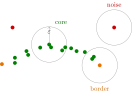
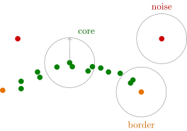
The three types of objects in DBSCAN with (a schematic, counting the object itself in its neighbourhood): green, core, with no fewer than objects in their -neighbourhood; orange, border, whose neighbourhood is not dense but who fall into the neighbourhood of a core one; red, noise. Circles of radius are shown for one object of each type.
How does the algorithm work? We take an arbitrary point. If it has a dense neighbourhood, we begin to consider each point of this dense neighbourhood and build an -neighbourhood around it too, and so on until we reach the boundaries of a certain set of objects. I like the analogy with a forest most of all here. Here is one forest, that is one cluster, and somewhere over there, across a clearing, another forest. We are in the forest and look: in our neighbourhood, as far as the eye can see, there are many trees, so we are at a core point. And we go on until we come out at the edge of the forest, and there we find ourselves at a border point: it is no longer core, there are fewer trees around, half of the space is already field, no forest. And somewhere there may be solitary trees; those are noise outliers. So we walk through the forest until we have gone round all of it, and as soon as we have, that is a cluster. Now we take a random tree and begin to build another cluster.
Definition (The DBSCAN algorithm). Input: a sample ; the parameters and .
Output: a partition of the sample into clusters and noise outliers.
- , unmarked; ;
- while there are unmarked points in the sample, :
- take a random point ;
- if , mark as possibly noise;
- else
- create a new cluster: ; ;
- for all that are unmarked or noise:
- if , then ;
- else mark as a border point of the cluster ;
- for all ;
- .
Let us write this algorithm as pseudocode, more precisely and strictly. At the start all points are unmarked; we will mark them by clusters. While there are unmarked ones, we take a random point. If its neighbourhood lacks density, we mark this point as possibly noise: it is certainly not core, but it is either noise or border, we do not know yet; later some noise points will turn into border ones. If the point turns out to be core, we put its neighbourhood into a new cluster, increase the number of clusters by one and begin to walk over this new cluster: for all points from the cluster that are unmarked or noise, if we see that the neighbourhood is dense, it means we keep walking through the forest, we are inside, we have not yet come out at the edge, and all the trees from the neighbourhood we again throw into this cluster, ascribe to this forest. If we have come out at the edge, we mark the object as border: we say that the tree at which we stopped is at the border of the forest. In this way we go round the whole cluster; if there is nowhere further to go, we have reached the edge everywhere we could, then all the objects we have placed in the current cluster get the label , and we exclude them from the unmarked ones. And we go through other forests.
Remark (The advantages of the DBSCAN algorithm).
- fast clustering of big data: in the worst case, with an efficient implementation of ;
- clusters of arbitrary shape (down with centres!);
- division of objects into core, border and noise.
What are the advantages and drawbacks of this method? The advantage, of course, is that it is very fast. One can reckon that in the worst case it is quadratic in the number of objects, but if there are efficient data structures for quickly building and traversing neighbourhoods, the algorithm becomes in complexity, which is really great and allows it to be applied to big data. The second advantage is that there are no centres. It works well on ribbon clusters and on clusters with bridges, in those cases I showed at the beginning that may be hard for simpler algorithms that just walk over the nearest objects, the so-called graph algorithms. I do not even tell about those; I consider them, after all, outdated. Clusters of arbitrary shape are great.
And it is great that we get a division of objects into three types. Core and noise, it is clear what they are. But the border objects should not be taken seriously: with them we do not mark out the boundary of each forest accurately. Where we came out at the edge, which random tree we ran into, that is what we marked as border. Other trees at the edge of the forest could have turned out to be border too; it just happened by chance that it was these. Some object is at the boundary but marked as core. This is not exactly a drawback of the method; it is simply that there is no question of accurately building the set of border objects. But the noise ones, please, they can be analysed further. This, of course, is a plus of the method: it gives an idea of which objects did not enter any of the clusters.
Here is DBSCAN; please welcome it. Many such algorithms have in fact been invented, but this one is perhaps the best known. DBSCAN and k-means are the best-known clustering algorithms, although k-means is not the best; I think I have explained why. And DBSCAN can be used practically always.
Hierarchical clustering
The Lance–Williams algorithm
Let us run on, to doing what Carl Linnaeus did, namely the problem of taxonomy, or hierarchical clustering. Here too I am telling an old algorithm; as you see, clustering was created mainly in the sixties and seventies, and these things are still used very actively. The Lance–Williams algorithm.
In hierarchical clustering there are in general two strategies: agglomerative and divisive. Agglomerative: we will gradually merge small clusters into larger ones, starting from individual points; this is what I am telling. Divisive: let us form large clusters and then begin to break them up into smaller ones; I am not telling this today, it is simply impossible to tell everything. So before you is the Lance–Williams method; it is agglomeration.
Definition (Agglomerative hierarchical clustering (Lance, Williams, 1967)). Iterative recomputation of the distances between the clusters , .
- , all clusters are 1-element;
- , the distances between them;
- for all ( is the iteration number):
- find in a pair of clusters with minimal ;
- merge them into one cluster: ; ;
- for all compute by the Lance–Williams formula:
What do we begin with? All clusters are one-element. Then at each step we find the two clusters nearest to each other and merge them into one; that is the whole idea, a very simple one. At each step the number of clusters decreases by one, and so step by step; at the last step the last two clusters will merge, and there will be one big cluster. We will decide later at which step we should have stopped and how many clusters to keep. Or we may not stop at all: we get a single hierarchical structure that shows how close different subsets of objects are to each other. How many merges are needed for all the objects to be in one cluster? ; so runs from 2 to .
We find the pair of clusters with minimal , merge them into one cluster, build the union, and say that the set of clusters now contains the union , while the two clusters that merged we exclude: the number of clusters in the set has decreased by one. One question remains, and it is the key one here, very interesting: since the clusters have merged, the distances between the merged cluster and all the others have to be recomputed somehow. The cluster did not exist before; it is a new finite set of points, and how is the distance between the finite set of points and another cluster to be computed? Off the cuff one can propose more than one or two ways: take the two farthest points, or the two nearest, or in each cluster in some sense the mean points and compute the distance between them, and one can invent a heap more such formulas. People in the early sixties, working on this problem, invented a heap of different formulas. And then Lance and Williams came and said: we give you one parametric formula with four parameters that very efficiently and easily recomputes the distance between clusters from the distances between the clusters that existed before the merge. is determined through three distances: , and . One has to know these three distances to compute the distance between the formed cluster and all the others we had before.
The question may arise: is such a linear form really enough? And what is this mysterious contraption, the absolute value of a difference, where does it come from? I will of course not give the proofs; I will give some explanations.
The Lance–Williams algorithm for semi-supervised learning
I promised to turn clustering algorithms into semi-supervised ones by correcting one line of code. Here is such a correction.
Definition (The Lance–Williams algorithm for semi-supervised learning). As in the hierarchical clustering algorithm, but at step 4: find in a pair of clusters with minimal provided that contains no objects with different labels.
We merge a pair of clusters only if they contain no objects with different labels. That is, we do not simply look for a pair of clusters with minimal distance but forbid taking pairs of clusters that contain objects marked with different labels: they will never merge, there is a strict ban here. We have introduced a separate if command into the algorithm, and that is all; nothing else needs to be done.
Special cases of the Lance–Williams formula
Now about the formula; this is of course the most interesting part. There are five special cases of the Lance–Williams formula, and behind each of them stands the proof of a theorem: some theorems are proved very easily, at once, while over some one has to sweat.
Definition (Special cases of the Lance–Williams formula).
- The nearest neighbour distance:
- The farthest neighbour distance:
- The group average distance:
- The distance between centres:
- Ward's distance:
Distances between clusters (slide): nearest neighbour, farthest neighbour, group average.
What first comes to mind when one wants to measure the distance between clusters? Let us take the nearest neighbours. It turns out that this is a special case of the Lance–Williams formula with these coefficients; a fact non-trivial at first sight, but in principle proved without difficulty; we will just not dwell on it now. And there are many little paradoxes here. It turns out that the nearest neighbour distance is almost the worst way of determining the distance between clusters as finite sets of points; the farthest neighbour distance works much better. Why this is so I will explain a little later. It too is a special case of the Lance–Williams formula. Or, for example, the group average: we take all the pairwise distances between points of one cluster and of the second, average them, and we have the distance between two finite subsets of points.
The distance between cluster centres (slide).
Now the distance between centres. If the points are elements of a linear vector space, we can compute centres: the operations of adding vectors and multiplying a vector by a number are defined. And in this case too the magic Lance–Williams formula works. One more paradox: this too is one of the worst distances, by certain criteria, I will tell you which in a moment; it is better not to take it. But if it is multiplied by a factor, we get a great distance, called Ward's distance; it works very well and is often recommended. And it too is a special case of the Lance–Williams formula.
The question arises: how to choose a better distance in this four-parameter family, and better by what criterion, and how can that be determined? Let us talk about the criteria.
The dendrogram
One of the criteria is hard to formalise: it is the clarity of the picture of the gradual enlargement of the clusters. One way of visualisation, the nesting diagram, is very inconvenient. When there are six points, it is seen splendidly: the nearest points merged into a cluster at the first step, the next ones at the second, the third step merged them together, and so on. But clearly, if there are even 60 points, you will get so tangled in these little circles that nothing at all will be visible. A bad way of visualisation. A good way of visualisation is called the dendrogram.
The nesting diagram and the dendrogram for the nearest neighbour distance (slide). The numbers at the ovals are the merge steps; along the vertical axis of the dendrogram are the distances at which the merges took place.
What do we see here? The first move: 3 and 6 merged, and the step shows the distance at which the merge happened, that very . The next move: 2 and 5 merged, at a greater distance, because at the very minimal distance we have already made the merge of 3 and 6. With the next move these merged, and here it is, the next step. With such U-shaped brackets we join the clusters that merge. About the process of drawing dendrograms one can also prove several theorems. The first: by choosing the ordering of the objects along the horizontal axis one can arrange that the brackets do not cross, provided that each next one is higher than the previous ones. This is important.
The nesting diagram and the dendrogram for the farthest neighbour distance (slide).
Let us see how other distances behave. The farthest neighbour distance: here too 3 and 6 merged first of all, but then the process of merging went differently, and the next bracket already made a different merge.
Remark (The dendrogram, a visualisation of hierarchical clustering).
- The clusters are grouped along the horizontal axis.
- The distances are plotted along the vertical axis.
- The distances increase; the lines do not cross anywhere.
- The upper levels are better distinguishable than the lower ones.
- The cut-off level determines the number of clusters.
The dendrogram is the thing for the sake of which agglomerative hierarchical clustering is done in the first place: it is done in order to build this visualisation; that is its aim. You have probably seen what trees are drawn in biology: species, subspecies, orders, classes and so on. And in many other problems the aim may be to make such a clear visual structure, and it is very important that it be convenient to look at: that all the U-shaped brackets do not cross.
And it is very convenient to draw a horizontal line: it shows where to carry out the clustering and determine the number of clusters. Why is it drawn precisely here? Because it seems that here is the largest gap between two successive brackets. Everything below are tightly packed clusters, because the distances at which the merges took place are much smaller; and everything above are large cluster structures, because the distances at which they merged are much larger. If we find the largest gap between the brackets, it will probably be the optimal number of clusters. In the picture on the slide we get seven of them, but one could draw the line higher and get three big clusters. It is a matter of our choice: the dendrogram is always built as a single one, in the end it joins all the points of the sample, and where to draw the division we can choose ourselves.
What would we like? That the lines nowhere cross; that the upper levels be better distinguishable than the lower ones. The fine grouping of points is perhaps not important to us, while the large-block cluster structure is more often important, so it would be great for the upper levels to be distinguished better than the lower ones.
Monotonicity, contraction and dilation
Can these "wishes" be formalised: we want a beautiful dendrogram, but what does beautiful mean? Such a formalisation was made, but not at once, note: the Lance–Williams algorithm is from 1967, while some of its properties and the properties of the dendrograms obtained were proved ten or even more years later.
Definition (The main properties of hierarchical clustering).
- Monotonicity: the dendrogram has no self-intersections; with each merge the distance between the merged clusters only increases: .
- A dilating distance: the differences grow.
- A contracting distance: the differences shrink.
The first property is monotonicity: we want the dendrogram to have no self-intersections. This can always be done if it is guaranteed that the distances at which the merges take place only grow. One more property, or rather two mutually exclusive properties: the distance is contracting or dilating. If the distances at which merging takes place are systematically smaller than the distances between the cluster centres, the distance is contracting: at the upper levels the merge levels differ from each other less and less, there will be a compaction upwards. And with a dilating distance it will be as in this picture: the compaction has stayed at the bottom, and further up the brackets are higher and higher. In most cases a dilating distance is more interesting to us, while monotonicity is always of interest to us.
Theorem (Milligan, 1979). The clustering is monotone if the conditions hold
is not monotone; , , , are monotone. is contracting; , are dilating.
The theorem is of course without proof; it is not very simple. The clustering is monotone if a system of four inequalities holds on the coefficients , , , which are checked completely elementarily, and one can say exactly that some distances suit us, they guarantee monotonicity, and some do not. For example, the distance between centres is not monotone, which is why I said it is not recommended. The nearest neighbour distance is contracting, so it too is not recommended. But the farthest neighbour distance and Ward's distance are dilating and monotone. Ward's distance is the most frequent recommendation, although it is not at all necessary to use precisely it: there are many combinations of the coefficients , , that satisfy the conditions of Milligan's theorem.
Remark (Ward's distance and the distance between centres). A question: is Ward's distance something like the distance between centres, only with "gravity" towards heavier clusters?
There was a great deal about this in the literature; precisely in the sixties and seventies people studied it; there is an amusing science of its own there, but by and large already done, and I do not want to go into it. There are other parametrisations too, for example a one-parameter one, which is also very often used in implementations of this algorithm, including in Python libraries.
The meaning of the factor can be understood like this. If a cluster of large cardinality and a one-point cluster merge, the factor is close to one, and Ward's distance is similar to the square of the distance between centres. And if both clusters are of roughly equal and large cardinality, the factor grows together with the cardinality, and the distance increases. That is, merging with a small cluster is encouraged more than merging two already powerful clusters. That is probably what it is about.
Recommendations and conclusions
Determining the number of clusters from the dendrogram (slide): Ward's distance; the cut-off line is drawn in the largest gap between successive merge levels; three clusters result.
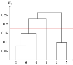
The dendrogram for Ward's distance with the merge levels taken from the slide (; ; ; ; ). The largest gap between successive levels is between and ; a cut-off line in it gives three clusters: , , .
Remark (Recommendations and conclusions).
- It is recommended to use Ward's distance .
- Usually several variants are built and the best one is chosen visually by the dendrogram.
- The number of clusters is determined by the maximum of ; then the resulting set of clusters .
I have already said all the recommendations and conclusions; I will repeat once more: Ward's distance is a good option. Usually several variants are built and the best is chosen, the one that, roughly speaking, satisfies the client more: what he wanted from his hierarchical clustering, what groups he expected to get. We can play with the Lance–Williams formula and then show several variants, and the client will say: I like this, I don't like that, for what reasons, God knows. And the number of clusters is determined by the maximum distance between successive brackets: we compare successive levels, and where the difference is largest, the division can be drawn and we learn how many clusters there are. Again, this is no optimality criterion at all, simply a heuristic: one can determine it this way, or in some other way.
Semi-supervised learning based on classification
Ahead there is still a whole interesting story: can classification methods be adapted for semi-supervised learning? Until now we have talked about the semi-supervised problem as a kind of side issue, usually a very light modification, correcting one line of code in a clustering algorithm; that has always been so. But can supervised learning methods, that is, classifiers, be adapted for semi-supervised learning? Yes, they can, and people also began working on this rather long ago, in the mid-sixties. I will tell three simple heuristic methods, and then more grounded approaches.
Self-training
Definition (The semi-supervised learning method self-training (1965–1970)). Let be a method of training classification; the classifiers have the form .
The pseudo-margin is the degree of confidence of the classification :
The self-training algorithm is a wrapper over the method :
- ;
- while :
- ;
- ;
- for all ;
- .
can be determined, for example, from the condition .
Suppose we have a method of training classification, and we need an estimate of the degree of confidence of the classification for an object that has no class label. If there were a class label, we would use the margin: the confidence in the correct class minus the maximal estimate of the degree of membership over all the other classes. Here is put instead of , because we do not know the true classification, and we get a pseudo-margin. The only thing we can substitute for the correct class is the estimate our current classifier gave, even if it is unreliable, built on a small set of labelled objects. Well, at least something. The pseudo-margin can already give us the objects on which we are so confident that, if the true stood instead of , the margin would be of the same sign and also large.
The idea of self-training is to gradually increase the size of the labelled sample, adding objects about which we are highly confident: that they belong to this class and hardly otherwise. We start from the sample of labelled objects, of which there are few, train some sort of classifier on them, take from this classifier a small number of objects on which the pseudo-margins are largest, consider that on them we have managed to determine the correct class, and simply add them to the sample .
Here are the two bananas as an example. There were only two objects, and some linear classifier passed somehow through them. Then we computed the pseudo-margins and said: these objects are so close to the red ones that we consider them reliably classified, and these are so close to the blue ones that they too are reliably classified, and we supplemented the training sample with them. It is clear what will happen with the next move: we will build a different classifier, then add more objects here and here, build a classifier again, and the objects will literally go round in a circle in this way one after another, and in the end we will separate our two bananas correctly. This is, of course, an advertising example, and things will not always go so well.
It is more reasonable to choose the threshold so as to label additionally, for example, 5 % of the objects each time; such is the heuristic. But this labelling is automatic; people no longer take part in it.
Co-training
Fine, but can the subjectivity connected with our using a particular model for classification be removed? Let us take two completely different methods, and they may be from different families: for example, one is the nearest neighbour method and the other a decision tree, so that their logic of working is absolutely different. Or these are two methods built on different sets of features, or even having different data sources. That is, they must complement each other in something, and they will teach each other.
Definition (The semi-supervised learning method co-training (Blum, Mitchell, 1998)). Let , be two substantially different training methods using
- either different sets of features;
- or different learning paradigms (inductive bias);
- or different data sources , .
- ; ;
- while :
- ; ;
- for all ;
- ;
- ; ;
- for all ;
- .
The process is very similar to the previous one. Each method in the general case has its own training sample. We additionally label the objects the first algorithm is confident in, that is , and use them to extend the training sample for the second algorithm. And vice versa: the second algorithm gives us reliably labelled objects, and with these objects we further train the first algorithm. They teach each other; hence co-training. Two students live in one hostel, one Chinese, the other Russian: the Russian teaches the Chinese Russian, and the Chinese teaches the Russian Chinese. Roughly such an analogy.
Co-learning
And can one go further and arrange that we have a heap of methods, as in boosting, many of them, and very different, and that they teach each other? People have invented a lot here, but one of the variants is quite simple: let us build a composition by voting, and then proceed in the same way as in self-training.
Definition (The semi-supervised learning method co-learning (de Sa, 1993)). Let be different training methods, . The co-learning algorithm is self-training for a composition, the simple voting of the base algorithms :
then is the degree of confidence of the classification .
- ;
- while :
- ;
- ;
- for all ;
- .
In fact one can invent a whole cloud more heuristics like the ones I have told. And it seems that these are some not very regular approaches: perhaps it works, perhaps it does not, perhaps it does not work in all problems. One wants something more grounded.
The general optimisation approach
Probably the most general approach to semi-supervised learning is in effect multi-tasking. There is a classification problem on the labelled sample, and for the labelled objects one can use classification loss functions. And there are unlabelled objects, and for them one can use loss functions for clustering. And a common model is built, a classification model. The criterion combines two criteria.
Definition (The general optimisation approach to SSL problems). Given: , labelled objects (labeled data) with labels ; , unlabelled objects (unlabeled data).
Find: a classification model .
The criterion of simultaneous classification and clustering:
where is the classification loss function, the loss function for unlabelled data.
The essence of SSL is a common parametrisation in two criteria.
The sample is divided into two subsets, labelled and unlabelled objects. The quality of clustering can, generally speaking, be measured on the labelled objects too, so the second sum here is written from one; one can also write it from ; in fact it is done both ways. It seems: why not use the labelled objects too in the criterion of clustering quality? Why not. The loss functions of these two parts of the problem are, naturally, different, and is a weight coefficient, as we have in regularisation, only here it is unclear who regularises whom: they have a common model with a common parameter vector, and they are, as it were, a kind of regularisers for each other. Moreover, there are situations where with such an approach the second problem is not clustering at all but some other problem with partial learning; we will get to such a variant too, we will consider it at the end.
Remark (Which loss functions to take). A question from the chat: is it implied here that the list of classes is known to us?
It may be either way; it all depends on how you build the criterion. The criterion of classification quality is, as we already know, some decreasing function of the margin: SVM, logistic regression, something of that kind. And for clustering you introduce a criterion that takes into account the specifics of the algorithm. The algorithm may require the number of clusters to be set in advance, and then one can write the k-means criterion, because it is an optimisation criterion. One can take the maximum likelihood, or the minimum of minus the likelihood, for a mixture of distributions, the same Gaussians, whichever you like: spherical, elliptical, of arbitrary form; this is the criterion optimised in the EM algorithm. Only now you will have a weighted sum of two criteria with the coefficient , and then the talk is about how to solve such an optimisation problem.
The transductive SVM
What has science invented on this topic? A really great method has been invented, based on SVM. Let us consider transduction as an example; for simplicity there will be two classes.
Definition (A reminder: SVM for two-class classification). A linear classifier for two classes :
The margin of the object :
The problem of training the weights , on the labelled sample:
The function penalises a decrease of the margin.
The idea: the function penalises an object for falling inside the separating strip.
We define the loss function for the classification problem; here it is, the piecewise-linear function of the margin. And now let us take not the margin itself but the absolute value of the margin. is , after all; when we take the absolute value, we no longer need to know . Wow, how great! Any loss function that depends on the absolute value of the margin, and, generally speaking, any even function of the margin, kills , and it no longer needs to be known for this object. And the loss function of such a thing, look: we begin to penalise an object for falling into the gap between the classes. What do we want? We want clustering, so a large gap between the classes, and few objects in this gap. That is precisely the criterion that we have done a clustering.
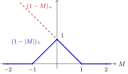
The loss functions of the transductive SVM: for labelled objects penalises a decrease of the margin; for unlabelled ones does not depend on the label and penalises an object for falling inside the separating strip .
Let us take an example. Suppose we have several labelled objects of the class "plus" and several of the class "minus"; from them one can see how the separating strip will pass; this is the ordinary SVM, and it will take in many unlabelled objects. If we began to penalise unlabelled objects in the strip, we would get not such a gap but this one, passing where there are no unlabelled objects.
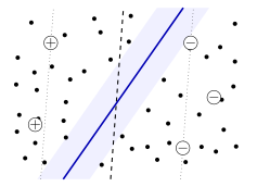
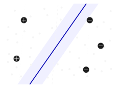
The transductive SVM (a schematic). The circles with plus and minus are labelled objects, the dots unlabelled ones. The dashed line is the separating line of the ordinary SVM trained only on the labelled objects (the dotted lines are the edges of its strip, inside which many unlabelled objects fall). The solid line and the shaded strip are the solution that penalises unlabelled objects falling into the strip: it passes through the region where there are no objects.
This is of course a demonstration example; it will far from always work out at all. If you try to solve a clustering problem and there is no cluster structure at all, it will give you nothing. But if there is a cluster structure, as here, you may get a substantially different position of the optimal separating hyperplane from the one the ordinary SVM would have given you.
Definition (The semi-supervised learning method Transductive SVM). Training the weights , on a partially labelled sample:
Merits and drawbacks of TSVM:
- as in the ordinary SVM, kernels can be used;
- there are efficient implementations for big data;
- the problem is non-convex, the optimisation methods are more complex;
- the solution is unstable if there is no region of sparsity;
- two parameters , have to be tuned.
Sindhwani, Keerthi. Large scale semisupervised linear SVMs. SIGIR 2006.
Let us write the functional and realise that optimising such a functional will differ little from optimising the standard SVM. For the labelled objects we have margins, for the unlabelled ones the absolute values of the margins, which do not depend on , and the regulariser. The merit is that, as in the ordinary SVM, the notion of support vectors works here, the sparsity of the solution and the possibility of an efficient implementation. Moreover, in many good libraries where SVM is implemented, TSVM is also present somewhere; perhaps it is buried in the documentation, it is not visible, but as a rule it is there. The drawbacks: the optimisation methods now become non-convex, a little more complicated; if there is no cluster structure, the solution may be unstable. And here two regularisation parameters also have to be tuned: in the ordinary SVM there was , and here one also has to weigh two criteria, on labelled and unlabelled data, and we get and , two parameters that have to be chosen somehow. Nevertheless such a contraption exists; in its time, when it appeared, it was a very interesting method.
Expectation regularisation (XR)
The last case I wanted to consider today should show you that the approach of optimising the sum of two criteria, one on labelled data and the other on unlabelled data, is much more general than clustering with partially classified objects, and can be used in much broader contexts. But to show this, let me first recall logistic regression, this time multiclass.
Definition (A reminder: multiclass logistic regression). A linear classifier over a finite set of classes :
The probability that the object belongs to the class :
The problem of maximising the regularised likelihood:
is optimised by the stochastic gradient method over the -dimensional parameter vector .
If there are many classes, the linear classifier is written as an , and for each class there is its own direction vector, which says: the farther you go in this direction, the more objects of the class there will be. Such a geometric interpretation. The training method optimises the directions for all classes at once. How are the parameters of the direction vectors to be converted into the posterior probability that the object belongs to the class ? This is done by the softmax function. The scalar product: the larger it is, the higher should be the probability that the object will be assigned to the class ; and the exponential with normalisation is a way of converting values of scalar products into values of probabilities. It is like how in two-class logistic regression the margin of an object is converted into the probability of correct classification through the sigmoid; it is a generalisation of the sigmoid. When we have posterior probabilities, we can use the maximum likelihood principle and write out the sum of the logarithms of these probabilities over all labelled objects. This likelihood has to be maximised, and it depends on the totality of parameters , over all classes together. One can also add an regulariser, and we get the regularised likelihood; by analogy with SVM, is the regularisation parameter: the larger it is, the smaller the influence of regularisation, at once over the direction vectors of all classes. Then it is clear: this problem can be solved by the stochastic gradient method. This was just a reminder; we have talked about logistic regression more than once.
Now suppose we have unlabelled data, and about these objects only the features are known; let these features be binary. One can compute pairwise distances and cluster the unlabelled objects. But can this be useful for improving the quality of solving the classification problem, in some sense for making up for the lack of information? There are few labelled objects, not enough of them, but there is a sea of unlabelled ones with the same features. Can this help in any way?
Definition (Agreement of the model on labelled and unlabelled data). Let us take into account the unlabelled data . Let be binary features, . Let us estimate the probabilities in two ways.
- The empirical estimate on the labelled data :
- The estimate on the unlabelled data and the probabilistic model:
We maximise the likelihood of the probabilistic model approximating the empirical distribution .
Let us see. Let us estimate the probabilities of the classes by individual features: the probability of the class given that the -th binary feature is present in the object, that is, equals one. The first thing that comes to mind is to compute it on the labelled data, no problem: in effect we make an estimate of a conditional probability. It may be simply a sample, empirical estimate: the share of objects of the class among all objects of the sample on which the -th feature equals one.
Is this the only way to make such an estimate? No. Let us substitute into this formula, instead of the knowledge of on the labelled objects, the estimate of the probability of on the unlabelled ones. We do have such an estimate: we are building a probabilistic classification model, the probability of a class for an object with parameters . Let us use it to estimate the conditional probabilities of the classes for each -th feature as well. The formulas differ little, only in that instead of the indicator of the class there is its probability, and the sums are computed over the unlabelled objects. This is another way of estimating the same conditional probabilities.
Now: these estimates should agree with each other, ideally. After all, they are computed in completely different ways and on different data, on labelled and unlabelled. Let us introduce an optimisation criterion that will make them agree. How is this done? By the maximum likelihood principle, of course. Why? Because some estimates depend on the model , while the others are empirical and are computed simply on the labelled data.
Definition (Building the regulariser (XR, eXpectation Regularization)). The log-likelihood of the model of the classes by the -th feature:
Regularising the criterion by the sum of the log-likelihoods with the regularisation coefficient :
Mann, McCallum. Simple, robust, scalable semi-supervised learning via expectation regularization. ICML 2007.
The model has the parameter , and in principle all such criteria have to be maximised for each -th feature. We write out the sum over all features: under the logarithm we have substituted the model estimate, and as weights the empirical one. And this is the criterion we had before for the same parametric multiclass classification model. And here we have got an optimisation problem in which, on an equal footing, there is still the sum over the objects of the sample, only for the labelled objects the loss function is like this, while for the unlabelled ones the loss function is more complex, a different one: it forces the model's conditional class probabilities for the features to agree with the empirical ones. But we get a functional of the same parameter , so we can optimise over the parameter in effect two different problems at once. How to optimise? As before, by the stochastic gradient method.
The authors of the method are two very well-known people in the field of text analysis, text classification, among the leaders. This was already almost twenty years ago, but they are nonetheless very respected people. They gave the method a rather strange name: expectation regularization, XR.
Remark (Features of the XR method (eXpectation Regularization)).
- XR is SSL, but it is not clustering at all!
- Optimisation by the stochastic gradient method.
- Possible ways of setting the variables :
- , then is the prior probability of the class (label regularization); suitable for problems with imbalanced classes;
- ; suitable for text classification problems.
- The method is weakly sensitive to the choice of and ,
- robust to errors in estimating ,
- does not require a large number of labelled objects ,
- is well suited to text categorisation.
XR is semi-supervised learning, but not clustering: there are no distances between objects here, no cluster structure, but simply information about the features, binary ones at that, of the unlabelled objects is used. And what are these binary features in the case of texts? That some word or term occurs in the text: each feature is the presence or absence of a term in the text.
And they invented one more variant: one can take simply a constant as . It would seem, what nonsense, it is uninformative, the constant one. But what do we get given that it holds? It is the prior probability of the class. And agreeing the estimates of prior probabilities is useful for imbalanced classes, when objects of some class number literally a handful: making a model that would know about this class imbalance is a good idea. And here this idea is implemented very easily, simply by adding a constant feature. The main features are the presence of a word in the text, and one more constant feature is introduced that takes care of evening out the classes, solving the problem of class balance.
Conclusions
Remark (Summary).
- Clustering is unsupervised learning, an ill-posed problem; there are many optimisation and heuristic clustering algorithms.
- DBSCAN is a popular fast clustering algorithm.
- The SSL problem occupies an intermediate position between classification and clustering but does not reduce to them.
- Clustering methods are easily adapted to SSL by introducing constraints (constrained clustering).
- The adaptation of classification methods is more often implemented through optimising a weighted sum of two criteria.
- SSL is not necessarily clustering (an example is XR); the essence of SSL is precisely the common parametrisation of two criteria, different on labelled and unlabelled data.
I am telling the XR method because the idea "let us combine two criteria, one for labelled data and the other for unlabelled data, but build them so that they depend on one and the same model with the same parameters " has turned out to be very general and very productive. One can say that practically no substantive problem is solved nowadays without such a combination of criteria, including where deep neural networks are built for classifying texts, pictures and so on: more and more people use multi-criteria formulations of problems. We have now worked out this approach ideologically, conceptually, on the example of semi-supervised learning; in the second half of the course we will recall it at almost every lecture, when several criteria work at once.
No comments yet
Be the first to share your thoughts.