August 30, 2026 · Lecture · LibreTimes
Machine Learning 1. Lecture 9. Logical Classification Methods
Contents
- What this lecture is about
- Decision trees
- The greedy ID3 algorithm
- The branching criterion: the impurity of the class distribution
- Handling missing values
- The merits and drawbacks of the greedy strategy
- Greed overcomplicates the tree
- Pruning a tree
- Regression trees: CART
- Rule induction
- Step 1. Families of rules
- Step 2. Generating rules
- Step 3. Selecting rules in (p, n) space
- Step 4. Building a classifier from regularities
- Summary
- The 2020 lecture
What this lecture is about
Today's lecture is a fairly natural continuation of the third part of the previous one, where we talked about feature selection. Today, one more big paradigm in classification theory — logical methods, discovering logical regularities in data — and there we will need the feature selection techniques we looked at last time.
An important point: logical classification methods were among the first; people began creating them back in the fifties and sixties, but interest in them gradually decreased. It became clear that methods based on interpretable knowledge discovered from data are limited after all. The famous scientist Yann LeCun, who did a great deal in neural networks, formulated this as a dilemma: «Do you want an interpretable model, or the one that works?» But in recent years interest in such models has been returning: how to combine the seemingly incompatible — to make models that work as well as the most advanced neural networks and are at the same time as explainable as rule-based systems or decision trees? The interpretability and explainability of machine learning and artificial intelligence models have again become a popular research topic. In general, rarely does something that developed strongly in machine learning lose popularity and go away for ever: from time to time ideas return.
Definition (Interpretability and explainability).
- Interpretability — the passive interpretability of the internal structure of a model or of a prediction on an object.
- Understandability, Transparency — the clarity, self-evidence, transparency of the model's structure.
- Explainability — actively generating an explanation on an object as additional output of the model.
- Comprehensibility — the ability to present the learned regularities as knowledge understandable to people.
When speaking of interpretability, people mean different things. Today we are talking about models that are interpretable passively: their very structure is clear and self-evident. Another option is explainability: a model may be very complex, like a neural network, but able to generate an explanation of why it made a decision on a particular object. We will not talk about that today; I have a separate lecture on it in the second semester. Today, interpretable models based on logic, on the attempt to extract human logic from data.
Decision trees
Let us start with a classical method — decision trees. These are classification algorithms specified by a tree. A tree is a connected acyclic graph; it always has a root, and its set of vertices divides into internal ones, which have children, and leaves, which have none. But it is not just a graph, it is a graph with additional information.
Definition (Decision tree). A decision tree is a classification or regression model specified by a tree (a connected acyclic graph) with root and set of vertices ;
- is a discrete feature, ;
- is the set of children;
- is the answer in the vertex .
The classification algorithm:
- ;
- while : ;
- return .
In practice binary features of the form , , are often used. If , the decision tree is called binary.
With each internal vertex a discrete feature is associated — a function of the object: at each vertex a discrete-valued feature can be computed from the object . And at the same vertex there is the function , which, from the value of the feature, says which child to go to next. The decision algorithm is very simple. Having an object , you stand at the root of the tree ; at the current vertex you compute the value of its feature and from it determine which child to go to; and so on until you reach a leaf. In the leaf there is a class label — an element of the set — and you return it. The main question, of course, is how to build such structures from a training sample.
Most often the features are numerical, and at a vertex a numerical feature is compared with a threshold: this is the most frequently used construction for building binary features. People also speak of binarization of the data: the original numerical features are turned into binary ones so as to branch on them. If all the features in a tree are binary, the tree is called binary: each internal vertex has exactly two children, a leaf has none, and there cannot be one child.
A decision tree for Fisher's iris problem and the corresponding partition of the feature plane (slide).
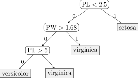
A decision tree for Fisher's problem of classifying iris flowers into three classes (50 objects of each class, 4 features). PL is the petal length, PW the petal width. In the axes of these two most informative features two classes separate without errors, and on the third there are 3 errors.
An example is Fisher's hackneyed textbook problem of classifying iris flowers. If the sample is drawn in the axes of petal width and length, one sees that the red class, setosa, separates well at once. Then it is not hard to separate the other two classes from each other. With a decision tree this is done very simply. The first condition is a horizontal line: if the petal length is less than 2.5, it is setosa. Then we draw a second line and separate most of one class from the other, and finally one more small correction. The problem has been solved quite well: literally a handful of objects of the training sample are misclassified, and the tree came out quite compact.
The greedy ID3 algorithm
Now let us work out how to build such trees. The recursive algorithm is called ID3. Everyone refers to John Ross Quinlan, to his 1986 paper «Induction of Decision Trees». But he did not invent it: all this was being invented back in the fifties and sixties, and by the mid-eighties a huge number of different algorithms had been devised. Quinlan generalized them and wrote a very clear text. People began to read it and cite it, because it was clear not to specialists but to people who use such algorithms in various subject areas — psychology, medicine, geology and so on.
Definition (Training a decision tree: ID3 (Iterative Dichotomiser)). The training sample , the features .
— the function calls itself recursively.
(input: ) output: the root of the tree :
- — the branching criterion of the tree;
- if , then create a new leaf ; ; return ;
- create a new internal vertex with the function ;
- for all :
- ;
- ;
- return .
The majority rule: .
John Ross Quinlan. Induction of Decision Trees // Machine Learning, 1986.
The TreeGrowing procedure builds a tree from a sample exactly as we have just done intuitively in the iris problem; but we need criteria by which to draw these lines, so that the parts of the sample are classified as well as possible and the tree comes out as simple as possible. As input the procedure gets a sample , and as output it gives the root of the built tree. The first time it is the whole training sample, but later the procedure will be called on subsamples. It looks for the feature that splits the sample into parts most profitably — into two if the tree is binary, though in general a feature may also branch non-binarily. We look for the feature that gives the maximum gain, the information gain from such a split of the sample; how this function is built we will work out a little later.
If the gain is less than the threshold , we say we will not split further: we create a leaf and write into it the label of the class most frequent in the sample — by majority vote. For example, when we immediately separated setosa without errors, a leaf arose at once: there is no point splitting further. If the gain is large enough, we create a new internal vertex and write the feature found into it. The feature takes several discrete values, and there will be exactly as many children, as many paths to descend further. So we go through all the values of the feature, build the subsample — all the objects of on which the feature takes the value — and feed it to the same function, so that it splits it further and builds the tree. Each subtree has been built by the TreeGrowing function, which returned its root; we hang this root as a child of the vertex and return . «Optimally» is of course in quotation marks here: there is no question of optimality; we look for the best option among those that seem best now.
The branching criterion: the impurity of the class distribution
How do we define the Gain function? First let us agree on a frequency estimate of the conditional probability of the class on the sample — the share of the objects of the sample belonging to the class :
Which distributions are most favourable for us? Those in which all the objects of the sample belong to one class. And what we like least is a uniform distribution of classes: it is maximally uncertain, or maximally «impure». Let us introduce a measure of the uncertainty of a distribution — impurity — that we want to minimize, and define it axiomatically.
Definition (The impurity of a class distribution). is the impurity of the distribution :
- it is minimal and equals zero when ;
- it is maximal for the uniform distribution ;
- it is symmetric: it does not depend on renumbering the classes.
satisfies these requirements, where the function is decreasing, non-negative, :
For example, the functions , , will do.
The measure is minimal and equals zero when one of the classes has probability one and all the others zero — we have determined the class precisely; this is the best case. The worst is the uniform distribution. And the measure must not depend on renumbering the classes. The other distributions are between the degenerate and the uniform. With such a definition a huge freedom of choice remains, and let us use it: let us choose a construction that is additive over the objects of the sample — a sum over objects of some loss function, minimizing which we are used to. Let us define as the expectation of the loss function of the class probability. The function must decrease — that is clear from the first two requirements. Substituting the frequency estimate into the definition of expectation, we get a mean over the objects of the sample: for each object we look at which class it belongs to and substitute that class into . If decreases, is non-negative and , it is easy to prove — I will not do it — that this function satisfies all three axioms. The construction is defined up to an arbitrary such function : minus the logarithm, , and many others will do. We cannot think of any additional requirement to define it more precisely, so we remain with this indeterminacy — perhaps these functions do not differ much anyway.
Now let us return to the ID3 algorithm, to the step where the feature that best splits the sample into subsamples by its values is chosen. Knowing the feature changes our uncertainty: instead of one distribution over classes, distributions in the subsamples arise, which may carry more information about the class, and the impurity measure will become smaller. We want to choose the feature that gives as much information about the class distribution as possible. The impurity given the feature is a sum that can be rewritten over the subsamples: the sum over is nothing other than up to normalization. The factor is a frequency estimate of the probability that an object goes from the parent vertex to the th child. That is, the impurity given the feature is the expectation of the impurity over the children, and the gain from branching is the difference of the impurities before and after choosing the feature:
The larger this difference, the more we have learned about the classes from the feature .
Example (Branching criteria: entropy, Gini). Two classes, ,
- If , then is the entropy of the sample.
- If , then is the Gini impurity.
The entropy criterion and the Gini impurity for two classes (slide).
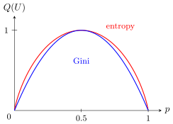
The impurity of a two-class distribution as a function of the share of one class: the entropy (red) and the Gini impurity (blue). Both are zero at and maximal at .
If we choose , everything we have done turns out to be equivalent to a difference of entropies from information theory. Historically, people first used information theory, computed entropies and derived these formulas, and a little later it became clear that the approach can be generalized — to the axioms of impurity I have shown. If we choose the function a little differently, is computed quite simply; it is a piece of a parabola. And it is interesting that this piece of a parabola leads to the criterion called the Gini impurity, and it is the one most often used in practice. Why? Purely computationally: when building large trees, computing logarithms begins to take substantial time. The entropy criterion that follows from information theory is of course better justified, but in the two-class case the entropy and the Gini impurity are very similar, and Gini is much simpler to compute. So at the dawn of these methods entropy criteria were used, and now, thanks to its computational efficiency, the Gini criterion is used.
Remark (How the threshold is chosen). Someone asked: first we go through all the features, for each we find a separating line, compute what information gain it gives, and choose the best among them all? Exactly right: the maximization in ID3 goes through the features and chooses the one that gives the maximum gain. Why did we separate setosa at once in the irises? Because that is the maximum gain: a class could be singled out entirely; the distribution over classes turned out degenerate. And it is not necessary to separate one class from the rest: if out of two hundred classes a hundred could be separated from all the others, that too is great — at the next levels we will start working inside this hundred.
And how is the optimal boundary determined? Our features are binarized, and if a feature has the form , the search is organized as two nested loops: first over all the features , and for each over the thresholds . The binary features need not be generated explicitly; we go through a list of thresholds. How to build this list — there are many options. If the training sample has a million objects, a million thresholds could in principle be gone through, but there is no need. The grid of thresholds should be neither too coarse nor too fine: the less we go through, the faster it works, but we may miss better threshold values. On the other hand, optimality is out of the question, because the algorithm as a whole is greedy, and determining the thresholds too precisely does not make much sense: even if they are chosen coarsely, nothing terrible will happen — terrible things happen anyway because of the greediness of the whole algorithm.
Handling missing values
What if not all the features of an object have been measured? This is a typical situation, for example, in medical diagnosis, where the features are symptoms, test results, and clearly it is impossible to measure in each person everything that can be measured. Sparsity is a natural property of medical data, and when building an algorithm for diagnostic decisions we will face the fact that the value of a feature sitting in the tree is undefined on a given object.
Definition (Handling missing values). At the training stage the following probabilities are estimated:
- — of going to from ;
- — of the class in the leaf ;
- if is undefined, then is excluded from when computing .
At the classification stage: is the most probable class, where
- if the value is undefined, then by the law of total probability ;
- otherwise .
At the training stage everything is clear: an object with an undefined value of the feature is simply excluded from the sample, and the gain is computed on the rest — there will be enough of them anyway to build the branching. We also remember the frequency estimates of the probabilities of going from the parent vertex to the children: they will be needed later. And in the leaves we compute the frequency estimate of the class probabilities over all the objects that reached the leaf. A subtle point: for this estimate to be unbiased, it is very desirable to estimate the probabilities on a held-out control sample, but as a last resort it can be done on the training one, only more carefully.
The most interesting part is at the classification stage. The algorithm is now probabilistic: arg max of the probability of the class given . Where do we get the distribution over classes at the root, if by the formula it is defined only in the leaves? We have to agree on how to lift these estimates from the leaves up to the root. If the value of the feature at an internal vertex is undefined on the object being classified, we look into all the children and compute the expectation: we do not know the value of the feature, but we know with what probabilities objects from this vertex go to the children — we estimated them at the training stage. This is a recursive step: the distribution over classes at the parent vertex is computed from the distributions at all the children. And if the value of the feature is defined, we simply lift the distribution from the child we go to. And so on until we reach the leaves, where we can compute the distribution on the training sample, or better on the control one. Thanks to this simple technique, decision trees are very easily adapted to data with gaps.
The merits and drawbacks of the greedy strategy
Remark (The greedy top-down strategy: merits and drawbacks). Merits:
- interpretability and simplicity of classification;
- rules do not require scaling the features;
- data of different types are allowed (through binarization);
- gaps in the data do not lead to refusals to classify;
- the amount of computation is linear in the sample length, .
Drawbacks:
- the greedy strategy overcomplicates the structure of the tree and, as a consequence, leads to overfitting;
- fragmentation of the sample: the farther is from the root, the lower the statistical reliability of choosing , ;
- high sensitivity of the trained tree to noise in the data, to the composition of the sample, to the branching criterion.
The greedy top-down strategy is quite fast. It is good in that all the features are binarized, and the feature scaling that often has to be done for linear classifiers or neural networks, where differences in feature scales can strongly affect the coefficients and cause overfitting, is not needed. Here, by choosing thresholds, one can work with features of any nature: a binary feature is the simplest thing there can be, and coarsening any feature measured on any scale to a binary one is always very simple. One can work with data of different types and with data with gaps; that is great. The cost is linear in the sample size and the number of features. Any object will be classified; there are no refusals to classify. And it is possible to estimate the probability that an object belongs to a class.
But there are drawbacks too. The strategy is greedy, and building an optimal decision tree is an NP-hard problem; this has been proved: in general a full search of all the trees that can be built from the given set of features is needed. It is impossible: the number of trees is astronomical, and all methods of building trees are one way or another methods of heuristically cutting down exponential search. Another drawback is a consequence of greediness and of the sample being fragmented as one goes from the root to the leaves. The subsamples get smaller and smaller, and it is from them that we make decisions about choosing features at the internal vertices and classes in the leaves. The closer to the leaves, the less data is used for these decisions, and they come out statistically unreliable. This of course affects the quality of decision trees.
The main advantage of trees, though, is interpretability: if they are not too deep, they reflect the logic of decision making, of those same doctors for example. A patient with complaints comes to a doctor, and from the first complaints, even from the patient's appearance, the doctor starts asking clarifying questions — and thereby uses a kind of decision tree in their head. Experts in many subject areas, especially in the pre-computer era, used something very similar to a decision tree: depending on the previous answers, the next questions are no longer anything at all but limited by a reasonable choice. Building decision trees literally copies the decision logic experts use. This explains the advantages and popularity of decision trees in applied problems. But, as we see, the advantages turn into drawbacks too.
Greed overcomplicates the tree
Greed leads to no good: the greedy strategy may overcomplicate the structure of the tree. Let me show this on a very simple example, a textbook one in connection with neural networks — the «exclusive OR» problem, which cannot be solved by a linear classifier.
The optimal tree for the XOR problem and the result of ID3 (slide), with the corresponding partitions of the square.
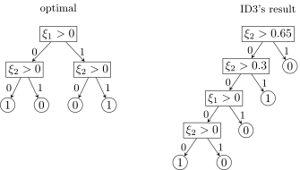
The XOR problem: the optimal tree of depth 2 (left) and the tree the greedy ID3 algorithm builds (right). The condition at the root of the optimal tree gives no gain on its own, and ID3 does not choose it.
The optimal solution here looks like a two-by-two chessboard and is obviously represented by a decision tree that we write out at once by looking at the picture. But can the ID3 algorithm determine that the sample should be split at once by ? Of course not: at the stage of choosing the feature at the root, such a split gives no information about the classes, no gain. The largest gain is given by a feature that separates the two top points from all the rest, and the building of the tree immediately goes wrong: everything after that goes askew, and we will not get the optimal tree. If we could look one step ahead and learn that after such a split the left and right parts can be separated like this, we would be happy — but ID3 cannot look ahead.
There were various strategies called look ahead. It turned out that they cope well with such artificial, showcase examples, but in general they make building a tree much more expensive. The complexity of building an optimal tree is in general exponential, and strategies that make the search, though not full, then wider, as a rule work better on a limited set of specially chosen examples and give little in practice. Look ahead was a popular research topic in its time but did not lead to big breakthroughs.
Pruning a tree
Another strategy, though, has stood the test of time — simplifying trees. Greed and its consequence, the fragmentation of the sample at vertices close to the leaves — statistically unreliable branchings and decisions in the leaves — lead to overfitting: trees come out excessively complex, with too many internal vertices, and work poorly on control data. What can be done about it? Prune the tree.
Definition (Pruning a tree: post-pruning strategies). is an independent control sample, .
for all :
- the subset of objects of that reached ;
- if , then replace by a leaf; ; exit;
- otherwise, by the minimum of the loss on control , choose:
- either replace by a leaf, ;
- or replace by a child subtree , ;
- or keep the whole subtree of the vertex .
Strategies for going through the vertices:
- bottom-up: Minimum Cost Complexity Pruning (MCCP), Reduced Error Pruning (REP), Minimum Error Pruning (MEP);
- top-down: Pessimistic Error Pruning (PEP).
For pruning, an independent control sample is usually used, a fairly large one: all the data is divided into three parts, two for training and one for control, because the control data will be used to estimate how good the subtrees are. For each internal vertex we look at which set of objects of the control sample reached the given subtree. If this set is empty, the whole subtree is statistically insignificant: the internal vertex should be replaced by a leaf and assigned a class by the majority rule — nothing better can be thought of here. If some control objects do get there, we try to understand what is better. The subtree can be kept whole. The main way of simplifying is to replace the subtree with one of its child subtrees: the quality of classifying the control sample will change, and if it improves, the replacement should be made. And the most radical way is to replace the subtree entirely by a leaf with a class by the majority rule. This general strategy is called post-pruning.
Why «post»? You first built an overfitted tree and then simplify it. A question arises: could the branching criteria not be made stricter and the tree built so that it comes out simpler straight away? The answer: this works worse than post-pruning; pre-pruning turns out to be a less profitable strategy. One should first build an overcomplicated, overfitted tree and then start simplifying it. No rigorous mathematical proofs of this have been found, but as an empirical fact it has been confirmed by many experiments.
In what order should the internal vertices be gone through — at random, bottom-up from the vertices close to the leaves, or top-down from the root? There is no single answer; there are many different strategies; I only list their names. Bottom-up strategies are used most often: we take the level next after the leaves, that is, the parents of the leaves, try to do something with them and gradually go up. But there is also the opposite, top-down strategy.
Regression trees: CART
Another modification often used in practice is the generalization of decision trees to regression problems. In fact it does not much matter which problem we solve, regression or classification, as long as we can define the branching criteria. Such a generalized model is called CART, classification and regression trees; people refer to Leo Breiman, 1984. Also fairly old things, but still applied.
What is a tree for regression? In general a tree is a piecewise constant function on the whole space of objects: it divides the space into regions (recall the picture with the irises). In a regression problem it remains for us to assign to each such region, that is, to each leaf , a value . Let us do it by least squares. Let be the set of objects that reached the vertex . The impurity measure is naturally defined as the mean squared error, and by minimizing it we find the value in the leaf.
Definition (CART: regression and classification trees). With the quadratic loss , , the least squares problem is solved analytically; the optimal value in the leaf :
A regression tree is a piecewise constant function.
Leo Breiman et al. Classification and regression trees. 1984.
We have already solved this problem several times — when we derived nonparametric regression, when we talked about loss functions in regression problems: the solution is the arithmetic mean of the over all the objects that reached the leaf. So a regression tree is a piecewise constant function whose value on each piece is the mean of the objects that fell there.
An example: regression trees of different depths for a simple one-dimensional sample — one numerical feature, with noise deliberately added to the data to show that on noisy data a tree tends to overfit. The more levels in the tree, the more complex the piecewise constant approximation becomes. Already at depth five leaves built from a single point appear, and if that point is an outlier, noise, it is clear overfitting. To fight it the Minimal Cost-Complexity criterion was invented.
Definition (CART: the Minimal Cost-Complexity Pruning criterion). The mean squared error with a penalty for the complexity of the tree:
As increases, the tree is successively simplified, and the sequence of nested trees is unique. From it the tree with the minimum error on the test (hold-out) is chosen.
The pruning problem can be posed here as an optimization one: the squared error plus a penalty for the number of leaves. How should the regularization coefficient be chosen? An interesting theory arises here, and several theorems can be proved: as increases, the tree is successively simplified, precisely by being cut back, and the sequence of nested trees is unique. By choosing from this sequence one can choose a unique tree, optimal, for example, by the hold-out criterion: since we are fighting overfitting, the quality of the trees must be estimated on held-out data. This is most often what is done. The method is also good in that the values in the leaves are computed analytically, as solutions of the least squares problem.
And once more the important thing: a tree is always a piecewise constant approximation of the original dependence, whatever problem we solve, classification or regression — a non-smooth, discontinuous function with steps. Not every problem suits such a solution, but sometimes a discontinuous function is quite acceptable.
Remark (Binary or non-binary trees). Someone asked: on quantitative data do we always use binary branching in trees? There was a big theoretical and applied argument about which trees are better: with large branching at each internal vertex or always with two children. It has been proved mathematically that binary trees are always enough: a tree with larger branching can always be represented as a binary one; that is practically obvious. In practice, in some problems, non-binary trees do work better. But binary ones are much easier to build, and binarizing features is the most convenient way of discretization, so binary trees took root in practice and are used most often. A final answer apparently does not exist in nature: it can be done either way.
Rule induction
The second part of the lecture is another big class of logical algorithms: rule induction algorithms, the search for logical regularities in classification problems.
Definition (A logical regularity). is the training sample, .
A logical regularity (a rule) is a predicate satisfying two requirements:
- interpretability: is written in natural language; depends on a small number of features (at most 7);
- informativeness with respect to one of the classes :
If , one says « selects » ( covers ).
A rule is a predicate, a binary function on objects, and there are two requirements for it, informal so far. The first is interpretability: the rule is written in natural language and, so that people understand it better, depends on a small number of features. Psychologists call this number the Yngve–Miller number, seven plus or minus two: that is how many items a person can keep in memory at once. The rules will later have to be shown to experts, and if a rule has 30 features, the expert will get confused and say «I do not understand this», while if it has two or three, at most seven, experts are willing to consider them and try to give them interpretations. The second requirement is easier to formalize: the rule should cover as many objects of its own class as possible — positive examples, — and as few objects of the other class as possible — negative ones, . Positive and negative — hence the letters and , easy to remember. We get a two-criterion optimization problem, and this creates a certain inconvenience; further on we will by hook or by crook turn it into a more familiar one-criterion problem.
Example (The interpretability requirement). From medicine. If «age > 60» and «the patient has had a heart attack», then do not operate; the risk of an adverse outcome is 60%.
From credit scoring. If «a home telephone is given in the application» and «salary > 2000 USD» and «loan amount < 5000 USD», then the loan can be granted; the risk of default is 5%.
Note. The risk is a frequency estimate of the class probability, computed as a rule on a held-out control sample.
Where do these risks come from? They are frequency estimates of the class probabilities on the set covered by the rule, where ; they can be made, for example, on a control sample. On historical data we computed the share of defaults among borrowers with such properties and saw that it is only 5%: the covered subset is reliable people with 95-percent probability. The intuition here is clear: in the pre-computer era too, people making decisions — the same medicine, the same bank analysts — worked out rules for themselves and wrote such systems of rules down explicitly. The most important property is that the analyst should understand all this, preferably remember it and use it at work. Building such rules from samples is what is called extracting knowledge from data, or rule induction: we try to derive the general from the particular. A huge number of algorithms have been invented, hundreds or perhaps thousands. This direction in machine learning probably began to develop before the others: the idea was first to extract rules from the heads of experts and build expert systems, and then to automate building them and pull rules directly out of data.
Definition (Training logical classifiers). The main steps of building rule induction algorithms — one has to specify:
- the family of rules in which regularities will be sought;
- a way of generating rules (rule generation);
- a criterion for selecting informative rules (rule selection);
- a classification model with the rules as features, for example a linear classifier (weighted voting):
In all such algorithms four main steps can be singled out. First, the form of the rules has to be fixed. Then we must learn to generate rules, of which some will be successful and others not. Agree on the criteria by which to select the successful ones. And finally, having gathered a large number of successful rules — and a rule is a function of the object, that is, a new binary feature — build some classifier over them: a tree, a linear classifier, even a neural network, but as a rule a linear one. Such constructions are called voting, in this case weighted: each rule votes for the class with its own weight. This is the most frequently used construction for logical algorithms, and in essence we already know how to build it: if binary features have been built and selected, we have already covered building a linear classifier on them. So the fourth step is in effect closed for us; let us deal with the first three.
Step 1. Families of rules
Definition (Frequently used families of rules).
- A threshold condition (decision stump): or .
- A conjunction of threshold conditions:
- A syndrome — at least of conditions holding (with it is a conjunction, with a disjunction):
- A half-plane — a linear threshold function: .
- A ball — a threshold function of closeness: , for example
- AVO, algorithms for computing estimates [Yu. I. Zhuravlev, 1971]: ;
- SCM, set covering machines [M. Marchand, 2001]: .
The parameters (, , , , , , ) are tuned on the training sample by optimizing a given informativeness criterion.
The most common way is threshold conditions on numerical features, as in the branching criteria of trees. The next, probably the most frequently used, is threshold conditions combined into conjunctions. It is very important that a small number of features is combined: the set is perhaps the main parameter here, the set of features to be looked at together. If together they satisfy some condition, then with high probability it is an object of a certain class. Conjunctive regularities are the most frequent way of discovering knowledge from data.
But medicine suggested another very interesting kind of regularity — syndromes. How does a symptom differ from a syndrome? A symptom is an original feature or, if the feature is numerical, a binarized condition: the indicator is within the norm, above or below the norm. A symptom of hypertension is high blood pressure. But to make a more or less reliable diagnosis, one has to know the symptoms of the disease, and in a particular patient you as a rule see not all of them but some subset. For example, a disease has ten symptoms, but if you see a combination of any four of them, you already say with great reliability: this is most likely such-and-such. Any four of these ten do not occur together just like that; each patient's illness runs its own course, in one some symptoms show more brightly, in another others, but if enough of them have shown up — of the set — it is reliable evidence of the diagnosis. A syndrome rule is something between a conjunction and a disjunction. Expecting to see all the signs of a syndrome at once is a conjunction, but that is too strict, and doctors say: you do not need all ten, four are enough. A disjunction is when one symptom is enough. It is not only doctors who think in syndrome rules: geologists, it turns out, do too when they search for mineral deposits, and many others.
Why does this work? Apparently, knowledge that took shape over centuries in various subject areas was accumulated by experts precisely in this form, so that it would be convenient for people to apply. That is why in these areas it is customary to measure features on which it is convenient for people to make decisions, and to build syndrome rules. This, it seems to me, is the only reasonable explanation of why syndromes so often turn out to be a successful way of representing knowledge.
Remark (What about feature weights?). Someone asked: feature weights suggest themselves too? Yes, but that is already fine tuning. A lot has to be optimized here anyway — both the set of features and the thresholds for each of them — and if weights are built in too, will there not be overfitting when you start training so many parameters? Methods for discovering regularities more often work on small data: in medical diagnosis, in geology, when searching for rare kinds of deposits, of which there are only a few or a few dozen known in the world, and there are only a handful of positive and negative examples. Searching for regularities in small data is a frequent situation for applying logical methods, and then there is no time for weights: it may not even be possible to tune them.
There are also more exotic families of rules. A half-plane is a linear classifier built on a small subset of features ; it must be small so that people understand how the rule works. This is exactly what brings methods of searching for logical regularities close to feature selection methods, and all the methods I told you about in the last lecture can be used here too. One can also use rules of the nearest neighbour type — balls: the predicate covers a neighbourhood of an object , a prototype of the given class, and says that everything around it at a small distance is also objects of this class. The distance is again defined on a small subset of features. In fact this is precedent-based thinking; it is characteristic of lawyers and doctors: I will make a decision because by this combination of diagnostic features my patient is similar to one I remember from my experience; that one had the same thing, and the treatment was successful. Such logic is understandable to people. Hence the requirement: in defining closeness, as in a conversation between experts, it matters by what combination of features this case is similar to that one. The weights can be trained, but when describing in the experts' language how a rule works, nobody will go into the details of choosing parameters; what matters is by what combination of features the closeness is built.
Step 2. Generating rules
Let us concentrate on conjunctions — they are the most frequent option. Conjunctions can be extracted directly from a tree.
Example (A decision tree → a covering set of conjunctions). The tree for Fisher's problem (figure above) gives four conjunctions, one per leaf:
Look how interesting. Take any leaf: how does an object get into it? Some condition along the way held, some did not, and we got into the leaf thanks to the conjunction of these conditions or their negations. In the end any leaf of any tree is a conjunctive rule, and the conjunction has exactly as many conditions as the length of the path from the root to the leaf. So a tree decomposes into a disjunction of conjunctions, and each object falls into one and only one of them: in classification any object falls into one and only one leaf. The conjunctions divide the whole space into disjoint regions — another useful property of a tree. If we build many different trees, we will build many sets of conjunctions that are guaranteed to cover the whole space: there will be no objects on which no conjunction ever returns one. This is a very good property: if conjunctions are optimized in any way whatever, uncovered regions of the space may remain, while a decision tree is wonderful in always covering the whole space simply by construction. There is a whole family of methods that pull conjunctions out of trees. But this is also bad: we did discuss that trees overfit.
Definition (Metaheuristics for searching for informative rules). Input: the training sample . Output: a set of regularities .
- initialize the initial set of rules ;
- repeat
- the set of local modifications of the rules from ;
- the most informative rules from ;
- while the rules keep improving;
- return .
Special cases (see the lecture on feature selection methods): stochastic local search; genetic (evolutionary) algorithms; beam search; depth-first search (branch and bound).
A huge number of algorithms for searching for regularities have been invented, hundreds if not thousands, and I tried to generalize them in a single pseudocode — this is indeed called a metaheuristic. First we generate some initial set of rules , at random even, then start applying local modifications to them, select the most informative among the rules and move to the new set; at the next iteration we again try to modify them locally. Special cases of this approach are the algorithms we considered last time, in the lecture on feature selection methods. There is one difference. There the criterion evaluated a subset of features, and it was an external criterion related to overfitting, and we were looking for one set of features. Here informativeness criteria of logical regularities will have to be used, and at the output many regularities have to be tuned, because a classifier will have to be built from them, as from binary features, at the fourth step.
Definition (Local modifications of conjunctive rules). The family of conjunctions of threshold conditions :
- varying one of the thresholds and ;
- varying both thresholds , at once;
- adding a feature to with varying of the thresholds , ;
- removing a feature from .
When a feature is removed (pruning), informativeness is usually estimated on a control sample (hold-out). In general, the same methods as for feature selection suit optimizing the set .
The most important thing is to add and remove features from the set . One can vary the thresholds, for example drop the lower or upper threshold. One can prune a conjunction — remove a feature, estimating the result on a control sample, just as we pruned trees. I will not tell these methods in detail: they can simply be applied once more, with two main changes — the external criterion is replaced by informativeness, and we look not for one optimal set of features but for as many sets as possible with decent informativeness values.
Step 3. Selecting rules in space
Now regularities have to be selected from the large number found. For now let us stay in the paradigm of two criteria: the number of own objects covered should be as large as possible, and of other objects as small as possible.
Definition (Two-criterion selection of rules in the plane). Positive: ;
negative: .
The Pareto front is the set of non-improvable regularities (a point is non-improvable if there are no points to the right of and below it).
This is called space: the number of positive examples is plotted along the horizontal axis, of negative ones along the vertical, and each point corresponds to one regularity. The best are in the lower right corner, but it is hard to get there: such a regularity alone would solve the problem without errors, and that is hardly achieved when the requirement of interpretability is imposed on the predicates. What is interesting here is the notion of the Pareto front, or Pareto-optimal front: the set of regularities that cannot be improved by both criteria at once. A point is non-improvable if there are no points to the right of and below it. There may be a dozen or a few dozen such points. Let us remove them from the plot and again single out the non-improvable ones — we get the second Pareto layer, then the third, the fourth and so on; this is called the Pareto layering of a finite set of points. Somewhere we will stop and perhaps throw out of the Pareto layers what does not suit us. For example, the edge where is large but is large too. Or the points where — wonderful — but is too small: these are simply statistically insignificant regularities. But a regularity that covered 50 own objects and zero others is great; such a feature can clearly be used.
Let me recall also the relative quantities by which the quality of logical regularities can be measured — precision and recall from the first part of the last lecture.
Definition (Logical and statistical regularities). A predicate is a logical regularity of the class if
If , then is a consistent regularity.
A predicate is a statistical regularity of the class if .
is minus the logarithm of the probability of the realization under the null hypothesis that and are independent random variables (Fisher's exact test):
where , , .
Logical regularities are selected by lower thresholds on precision and recall. If precision is 100%, the regularity is called consistent, but chasing such regularities makes sense far from always: their recall is, as a rule, low.
Can one criterion be assembled from the two after all? One way is to build statistical criteria and test statistical hypotheses. is a binary quantity, own class or other, and is also a binary quantity, whether the object is covered by the regularity or not. The null hypothesis is that these two random variables are statistically independent, that there is no relation between the rule and the target . Under such a hypothesis the probability distribution of the quantities and can be derived, and it is a known distribution — the hypergeometric one, and the test built on it is called Fisher's exact test. The test consists in computing the probability of a purely random realization of exactly such and , given that there are own objects and others. The smaller this probability for the observed , , the more strongly we contradict the null hypothesis of independence and the less random the relation between and . If we take minus the logarithm of the probability, the larger the better — and that is the statistical informativeness criterion. Normalization by is also often used.
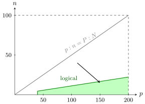
space with , (schematic). The diagonal is the rules that keep the class proportion: they carry no information. The farther from the diagonal towards the lower right corner, the higher the statistical informativeness (the arrow). The green trapezoid is the logical regularities, Precision , Recall .
How do logical and statistical criteria relate; where do they lie in space? There is a big difference between them. The diagonal is the worst regularities, whose and are in the same proportion as and : such rules give no information about the class distribution. The farther from the diagonal, the greater the statistical weight of the regularity. And a logical regularity rather strictly cuts off the lower part of space: precision above something, recall above something — that is the trapezoid at the bottom. These really are rules that make a small number of errors and at the same time cover quite a lot of objects, and their statistical informativeness is simply off the scale. But there is a large region of regularities that are statistical but not logical.
How should all this be viewed? Statistical criteria are more convenient in the process of searching for rules. When we gradually complicate the rules — add features to them, remove them — we travel around this space, and our task is to lead the rule points to the lower right corner. A statistical criterion is sensitive to where we are in this space, and in this sense it is most useful to us. And when we have already got into the region of logical regularities, we can say: we have found a reliable rule; it is a very good feature to use in a classifier. That is, the logical criterion is convenient for the final selection of rules that are interpretable individually, and then a classifier is built from them.
Definition (A zoo of informativeness criteria). Obvious but not quite adequate criteria:
- (precision);
- (recall);
- (relative accuracy).
Adequate but not obvious criteria:
- the entropy criterion of information gain:
where ;
- the Gini criterion (Gini impurity): with ;
- the boosting criterion and its normalized variant: , .
J. Fürnkranz, P. Flach. ROC'n'rule learning — towards a better understanding of covering algorithms // Machine Learning, 2005.
Let me refer to a rather old 2005 paper with a quite wonderful title, «ROC'n'rule learning». What has the ROC curve got to do with it? ROC curves and spaces are closely related: the lower envelopes here are a little like ROC curves in other coordinates, and so is the striving towards a particular corner — to the maximum, to the minimum. A huge number of criteria in space have been invented; I described one, Fisher's exact test, but more than twenty are described and compared in this paper. Precision and recall are expressed through and like this, and many other things can be invented. And one can build many counterexamples showing that however you try to aggregate and in different ways, there are always cases where it works badly. The adequate criteria are the entropy and Gini ones, those very Gain gains we defined for the branching criteria in trees; all this can be repeated in terms of and . I did not derive the formulas; they are easily derived, and these informativeness criteria work fairly adequately. There is also the interesting criterion ; we will talk about it in a few lectures, when I tell you about boosting — it is a rather amusing theory. But is bad; a counterexample can be built for it.
Example (Nontrivial problems of combining two criteria). In each pair of rules the first is much better than the second, yet simple heuristics do not distinguish them in quality (with , ):
| 50 | 0 | 50 | 50 | 0.25 | 50 | 22.65 | 23.70 | 7.07 |
| 100 | 50 | 50 | −150 | 0 | 1.96 | 2.33 | 1.98 | 2.93 |
| 50 | 9 | 41 | 5 | 0.16 | 5 | 7.87 | 7.94 | 4.07 |
| 5 | 0 | 5 | 5 | 0.03 | 5 | 2.04 | 3.04 | 2.24 |
| 100 | 0 | 100 | 100 | 0.5 | 100 | 52.18 | 53.32 | 10.0 |
| 140 | 20 | 120 | 40 | 0.5 | 6.67 | 37.09 | 37.03 | 7.36 |
Note. The criteria IStat and IGain are asymptotically equivalent: as .
Inventing a combination of the criteria and that would give a single convenient and correct informativeness criterion is a nontrivial problem; people struggled with it for several decades, and Fürnkranz's 2005 paper summed up this stage. Simple criteria do not stand up to criticism: pairs are found where the first is a good regularity and the second clearly no regularity at all, because it keeps the proportion , yet the criterion does not distinguish these two cases. But the statistical and entropy criteria, the Gini criterion, distinguish such situations more finely, and they can really be used for optimization in space.
Step 4. Building a classifier from regularities
Definition (Building a classifier from regularities). Weighted voting (a linear classifier with weights and, possibly, with regularization for feature selection):
Simple voting (a majority committee):
A decision list (a seniority committee), : the rules are queried in turn; the first rule that fires returns its class , and if none fired, is returned.
The last step of rule induction is building a classifier from the regularities. One can build linear classifiers with weights , or simply set the weights equal. Or another degenerate case — the decision list: all the rules are lined up in a sequence and queried one after another. This is precisely an expert system, a rule-based system. What matters, of course, is in which sequence to arrange the rules, but classifying is very easy. A decision list is a special case of a decision tree that has one long branch. How to build decision lists I no longer have time to tell; these too are greedy algorithms, but practically nobody uses them now — they are rather old methods of rather low quality, so you will lose little.
But what I will have occasion to talk about is so-called oblivious decision trees. They turned out to be a very successful construction: coarse, very quickly built, and convenient to build in large numbers and make a weighted vote of, that is, to assemble a linear classifier out of trees. This is the gradient boosting technique; MatrixNet, which was used for many years at Yandex for ranking and other machine learning problems, was built as a combination of such oblivious decision trees. How this contraption works I will tell in one of the next lectures. And the answer to the question of how to choose thresholds: there are separate algorithms for this too, dozens of them invented. It is a minor, auxiliary problem that is solved relatively easily.
Summary
Advantages: interpretability; the ability to handle data of different types; the ability to handle data with gaps.
Drawbacks: limited classification quality; decision trees are unstable and prone to overfitting.
Ways to remove the drawbacks: reduction on test data; compositions of rules, forests of trees (in the next lectures).
The lecture turned out dense, but the material is arranged so that the most important came first. Decision trees are technique number one, conjunctive regularities second in importance, and everything else is trimmings, small things and details.
No comments yet
Be the first to share your thoughts.