August 30, 2026 · Lecture · LibreTimes
Machine Learning 1. Generalization Theory
Contents
- What this lecture is about
- The problem of estimating generalization ability
- The error matrix
- The probability of overfitting
- The case of a single algorithm
- The principle of uniform convergence of frequencies
- The Vapnik–Chervonenkis bound
- Infinite families: the growth function and capacity
- Inverting the bound: the complexity penalty
- Structural risk minimization
- Why the Vapnik–Chervonenkis bounds are overstated
- The Occam's razor bound
- Summary
What this lecture is about
In the previous lecture generalization ability was estimated empirically — on a control sample, by cross-validation — or by analytic criteria of the form «internal criterion plus a complexity penalty», such as AIC, BIC and the Vapnik–Chervonenkis bound. Where do such penalties come from? The answer is given by generalization theory: it looks for upper bounds on an algorithm's quality on hidden, control data that can be computed from the training sample alone. The classic result of this theory is the Vapnik–Chervonenkis bound; from it come the notions of the growth function and the capacity of a family of algorithms, and the method of structural risk minimization. We will see how the bound is obtained, why it is heavily overstated, and how the Occam's razor bound leads to the regularization we already know.
The problem of estimating generalization ability
Definition (The problem of estimating generalization ability). Given:
- is the general set of objects;
- is a partition into training and control parts;
- is the model, a family of algorithms;
- is the training method;
- is the loss of algorithm on object ;
- is the mean loss on the sample .
Find: a way to estimate and minimize without knowing , for a wide class of problems and methods
under simplifying assumptions:
- the loss function is binary;
- all partitions are random and equally likely.
We want to know how the trained algorithm will behave on the control sample , which it did not see during training. We see only the training sample, yet we want to estimate the quality on the hidden one. To make the problem mathematically meaningful, two simplifying assumptions are made. The loss function is binary: on each object the algorithm either errs or does not. And all partitions of the general set into training and control are equally likely: none of them is singled out, and the observed part could have been any of them.
The error matrix
With a binary loss function, all we need to know about an algorithm is the objects on which it errs.
Definition (Binary loss function. The error matrix). is a finite general set of objects; is a finite set (family) of algorithms;
is the error indicator.
The error matrix is the matrix with pairwise distinct columns; the first rows are the observed (training) sample , the other the hidden (control) sample .
is the number of errors of on the sample ;
is the error rate of on the sample .
A column of the matrix is the algorithm's error vector. Two algorithms with the same error vector are indistinguishable for us, so the columns are pairwise distinct: they are no longer algorithms but equivalence classes of algorithms. Even an infinite family, such as linear classifiers with real weights, has a finite number of distinct error vectors on a finite sample.
Example (The error matrix of linear classifiers). For a sample of ten points on the plane, linear classifiers generate one error vector with no errors, five vectors with one error, eight vectors with two errors, and so on (the first 14 columns: has no errors, one, two):
| 0 | 1 | 0 | 0 | 0 | 0 | 1 | 0 | 0 | 0 | 0 | 1 | 1 | 0 | ||
| 0 | 0 | 1 | 0 | 0 | 0 | 1 | 1 | 0 | 0 | 0 | 0 | 0 | 0 | ||
| 0 | 0 | 0 | 1 | 0 | 0 | 0 | 1 | 1 | 0 | 0 | 0 | 0 | 1 | ||
| 0 | 0 | 0 | 0 | 1 | 0 | 0 | 0 | 1 | 1 | 0 | 0 | 0 | 0 | ||
| 0 | 0 | 0 | 0 | 0 | 1 | 0 | 0 | 0 | 1 | 1 | 1 | 0 | 0 | ||
| 0 | 0 | 0 | 0 | 0 | 0 | 0 | 0 | 0 | 0 | 1 | 0 | 1 | 0 | ||
| 0 | 0 | 0 | 0 | 0 | 0 | 0 | 0 | 0 | 0 | 0 | 0 | 0 | 1 | ||
| 0 | 0 | 0 | 0 | 0 | 0 | 0 | 0 | 0 | 0 | 0 | 0 | 0 | 0 | ||
| 0 | 0 | 0 | 0 | 0 | 0 | 0 | 0 | 0 | 0 | 0 | 0 | 0 | 0 | ||
| 0 | 0 | 0 | 0 | 0 | 0 | 0 | 0 | 0 | 0 | 0 | 0 | 0 | 0 |
There are few algorithms with a small number of errors, and as the number of errors grows there are more and more of them. This picture — one best algorithm, a few slightly worse ones, its neighbours, and still more that are worse still — is typical, and at the end of the lecture we will see that it is exactly what makes the classical bounds heavily overstated.
The probability of overfitting
Definition (Overfitting and the probability of overfitting). The overfitting of a method is the difference between the error rates on and on :
Overfitting as an event is .
The main probabilistic assumption: all partitions are equally likely,
Interpretation 1: this is CCV, complete cross-validation. Interpretation 2: this is the hypothesis that the sample is independent.
The main problem is to estimate the probability of overfitting:
is the empirical Monte Carlo estimate over a random subset of partitions.
Overfitting measures how much higher the error rate on control is than on training. Training minimizes the error rate on the training sample, so on control it is usually higher, and the question is by how much. The event «the overfitting is at least » is called overfitting, and we want to estimate its probability.
Probability here is understood combinatorially: it is the share of partitions of the general set into training and control on which overfitting occurs. On the one hand, averaging over all partitions is exactly complete cross-validation, which we discussed in the previous lecture. On the other hand, equally likely partitions are a weak form of the hypothesis that the sample is independent: if the objects are independent and identically distributed, no partition is better than another. Computing the sum over all partitions is usually impossible, but it can always be estimated by the Monte Carlo method, over a random subset of partitions.
The case of a single algorithm
Let us begin with the simplest but important special case: the family contains a single algorithm. Then there is no choice and no training, but the question remains: how much can its error rate on control differ from the rate on training?
Theorem. Let be a one-element set, . Then the probability of overfitting is the probability of a large deviation of the error rates of in two subsamples:
For any and any the probability of overfitting is given by the hypergeometric distribution function:
Proof.
-
Let be the number of errors of the algorithm on the training sample.
-
This is a «school» problem in probability: an urn holds balls, of them black; we draw balls at random. What is the probability that of them are black?
- Write out , substituting , :
since the condition is equivalent to .
The balls in the urn are the objects of the general set, the black balls are the objects on which the algorithm errs, and the balls drawn at random are the training sample. Overfitting happens when too few errors land in training and too many in control.
The hypergeometric distribution (slide): on the left at , on the right at , for all .
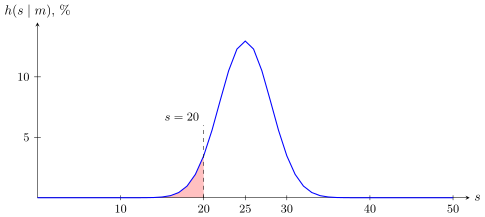
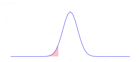
The hypergeometric distribution of the number of training errors at , , (computed exactly). The shaded tail is the probability of overfitting at : .
Remark (Concentration of the probability measure). Predicting the number from the number is possible thanks to the narrowness of the hypergeometric peak, and as it narrows further, so that . This is the law of large numbers in combinatorial form.
The distribution is concentrated around , that is, around the share of errors that falls into training in proportion to its length. The longer the samples, the narrower the peak relative to its position: the number of errors on training predicts the number of errors on control, and the more data, the more precisely. For a single algorithm overfitting is unlikely. The trouble starts when the algorithm is chosen from a family using the training sample.
The principle of uniform convergence of frequencies
Now let the family be arbitrary but finite. The training method picks an algorithm from it by looking at the training sample, and how exactly it does so is unknown. The classical theory gets around this difficulty in two steps.
Definition (Two upper bounds).
- Bound the probability of overfitting from above by the probability of a large uniform deviation of frequencies: for any ,
- Bound the probability of a union of events by the sum of their probabilities (Boole's inequality, the union bound):
The first step gets rid of the training method: whatever algorithm chooses, its overfitting is no greater than the maximum over the whole family. The bound holds for any training method — even the worst one, which picks exactly the algorithm that overfits the most. The second step reduces the problem to the case of a single algorithm: each term is the probability of overfitting of one algorithm, which we already know how to compute exactly.
The Vapnik–Chervonenkis bound
Substituting the hypergeometric formula into the sum gives a lemma, and bounding each term by the worst one gives a theorem.
Lemma. For any , , finite and
Theorem (Vapnik and Chervonenkis, 1968). For any , , finite and
V. N. Vapnik, A. Ya. Chervonenkis. On the uniform convergence of relative frequencies of events to their probabilities. 1968.
The probability of overfitting decreases exponentially as the sample grows, but grows in proportion to the number of algorithms in the family. The richer the family, the more likely it is to contain an algorithm that happens to fit the training sample well and works poorly on control. This is the quantitative form of the effect that excessive model complexity leads to overfitting.
Infinite families: the growth function and capacity
For infinite families, such as linear classifiers, and the bound becomes meaningless. But on a finite sample there are finitely many distinct error vectors, and only they matter.
Definition (The growth function and capacity). The growth function of a family is the maximum over of the number of distinct error vectors . In the Vapnik–Chervonenkis bound, can be replaced with the growth function .
The capacity (Vapnik–Chervonenkis dimension, VC dimension) of a family is the largest sample length for which .
As long as the sample length does not exceed the capacity, the family can realise all error vectors on it — separate the points in any way. Beyond that the growth function stops growing exponentially.
Theorem. If such an exists, then
Theorem. The capacity of the family of two-class linear classifiers
equals the dimension of the parameter space: .
The growth function of a family of finite capacity grows polynomially in , while the probability of overfitting decreases exponentially in , so their product still tends to zero: a family of finite capacity is learnable. For linear classifiers the capacity is simply the number of features; for more complex models estimating it is a nontrivial combinatorial problem.
Inverting the bound: the complexity penalty
The probability bound can be inverted: setting its right-hand side equal to a significance level and solving for , we get a bound on the error rate on control that holds with high probability.
Theorem (Inverting the Vapnik–Chervonenkis bound for ℓ = k).
- If , then for any with probability at least
- If , then for any with probability at least
This is the very Vapnik–Chervonenkis bound that appeared among the analytic external criteria in the previous lecture: the error rate on control is at most the rate on training plus a complexity penalty. The penalty grows with the capacity roughly as and decreases with the sample length. It can be computed without seeing the control data, and the whole sample goes into training.
Structural risk minimization
The inverted bound immediately gives a method for choosing a model of optimal complexity. If the families can be ordered by increasing capacity, pick the one on which the sum of the empirical risk and the complexity penalty is smallest.
Definition (Structural risk minimization (SRM)). Given: a system of nested subfamilies of increasing capacity
Find: the optimal capacity such that
Drawbacks of SRM:
- the upper bound on is very heavily overstated;
- consequently, may come out too low;
- in practice empirical CV estimates are preferred.
V. N. Vapnik, A. Ya. Chervonenkis. Theory of Pattern Recognition. Moscow: Nauka, 1974 (in Russian). V. N. Vapnik. Estimation of Dependences Based on Empirical Data. Moscow: Nauka, 1979 (in Russian).
As grows, the first term decreases — a richer family contains an algorithm better fitted to the training sample — and the second grows. Their sum has a minimum, and this is the same picture as for the external criterion in the previous lecture: a characteristic minimum over model complexity. For example, may be the linear classifiers that use the first features; then SRM is feature selection by an analytic external criterion. The trouble is that the bound is very heavily overstated, the penalty comes out too large, and the optimal complexity comes out too low. That is why in practice empirical estimates — cross-validation — are used more often.
Why the Vapnik–Chervonenkis bounds are overstated
The derivation of the bound had two steps, and each of them can overstate the result heavily.
- The uniform deviation bound (uniform bound) is heavily overstated when most algorithms have a vanishingly small probability of being the result of training. In practice the distribution , , is as a rule far from uniform. We will call this the splitting effect of the family .
- Boole's inequality (union bound) is heavily overstated when many of the binary error vectors are alike. We will call this the similarity effect of algorithms.
K. V. Vorontsov. Splitting and similarity phenomena in the sets of classifiers and their effect on the probability of overfitting. 2008.
The first step replaced the chosen algorithm with the worst one in the whole family. But the training method minimizes the error on the training sample and almost never picks algorithms with many errors — and it is exactly those that make up the overwhelming majority of the family; recall the error matrix of linear classifiers. The family splits, as it were, into layers by the number of errors, and only its bottom layer really works. The second step bounded the probability of a union of events by the sum of probabilities, as if the events did not intersect. But for similar algorithms, whose error vectors differ on one or two objects, the overfitting events almost coincide, and the sum counts the same thing many times over. In real families — linear classifiers and many others — the algorithms as a rule form connected sets of error vectors similar to one another. Accounting for both effects is the subject of the combinatorial theory of overfitting.
The Occam's razor bound
How can at least the splitting effect be accounted for? We cannot know the distribution , but we can try to «guess» it.
Theorem (Langford, 2002). For an arbitrary normalized function , , any and any , with probability at least
Statement 1. If we guessed right, , then is minimal.
Statement 2. Occam's razor can account for the splitting effect but not the similarity effect, so it is overstated too.
John Langford. Quantitatively tight sample complexity bounds. 2002.
Now the complexity penalty is individual for each algorithm: the larger the prior weight we assigned to the algorithm before seeing the data, the smaller its penalty. Algorithms we considered plausible in advance are penalized lightly, the rest heavily. Hence the name: Occam's philosophical principle says not to multiply entities beyond necessity, that is, to prefer simple explanations — and the bound does favour simple, a priori more probable algorithms. How should be set? Let us look at two examples.
Example (The uniform distribution gives the Vapnik–Chervonenkis bound). is a finite set. The uniform distribution gives the Vapnik–Chervonenkis bound: for any , , with probability at least
If we know nothing about which algorithms will be chosen and consider them all equally likely, Occam's razor turns into the Vapnik–Chervonenkis bound for a finite family. In other words, the Vapnik–Chervonenkis bound is Occam's razor with the worst, uninformative guess about the distribution .
Example (The Gaussian distribution gives regularization). Two-class classification, ; are the linear classifiers in :
The Gaussian distribution: the weights are independent random variables with zero mean and equal variances :
where is a normalizing factor independent of . Substituting into the «Occam's razor», we get… regularization!
The complexity penalty turned out to be an increasing function of the squared norm of the weight vector. Minimizing the right-hand side of the bound means minimizing the empirical risk while keeping the weights from growing: this is regularization, which we have already met from considerations of solution stability and from the probabilistic interpretation — as a Gaussian prior on the weights. Generalization theory leads to it from a third side: regularization lowers the upper bound on the error rate on control data.
Summary
- The generalization ability of a training method is measured by the probability of overfitting — the share of partitions of the general set on which the error rate on control exceeds the rate on training by more than .
- For a single algorithm this probability is computed exactly through the hypergeometric distribution and decreases quickly as the sample grows.
- For a family of algorithms the classical theory bounds it from above by the probability of a uniform deviation of frequencies and by Boole's inequality. This yields the Vapnik–Chervonenkis bound, in which the complexity of the family is measured by the growth function or the capacity.
- The inverted bound has the form «empirical risk plus a complexity penalty»; structural risk minimization is built on it.
- The bounds are heavily overstated because of the splitting and similarity effects. Occam's razor accounts for splitting through the prior distribution and in special cases gives the Vapnik–Chervonenkis bound or regularization; accounting for both effects is the subject of the combinatorial theory of overfitting, to which a separate lecture is devoted.
No comments yet
Be the first to share your thoughts.