August 30, 2026 · Lecture · LibreTimes
Machine Learning 1. Lecture 8. Feature Selection, Model Evaluation and Model Selection
Contents
- What this lecture is about
- Measures of classification quality
- The ROC curve
- Gradient maximization of AUC
- The log-likelihood for a probabilistic model
- Precision and recall
- The multiclass case: micro- and macro-averaging
- ROC and Precision–Recall curves
- Generalization ability and external criteria
- The problem of choosing a model and a learning method
- Internal and external criteria
- Empirical external criteria: cross-validation
- Model consistency
- Analytic external criteria: regularization
- Multi-criteria model selection
- Feature selection by an external criterion
- Full search
- Greedy addition
- Alternating addition and deletion
- Depth-first search and branch and bound
- Beam search (GMDH)
- Evolutionary algorithms
- Random search with adaptation
- Summary
- Seminar
What this lecture is about
Today's topic is classification quality, generalization ability and feature selection methods. In fact this would stretch to two or even three lectures, but everything had to be combined: there are other things that need lectures of their own. The lecture will have three parts. First, how to evaluate classification quality; it would seem there is nothing to talk about, but many pitfalls lie here. Then, what generalization ability is and by which external criteria it is evaluated. And finally, armed with external criteria, we will take up feature selection.
Measures of classification quality
Let us start with evaluating classification quality. Consider a problem with two classes, , as we did before. Four cases are possible, and I give the terminology straight away in a table.
Definition (Type I and type II errors). A two-class classification problem, ; a classification algorithm .
| the classifier's answer | the correct answer | |
|---|---|---|
| TP, True Positive | ||
| TN, True Negative | ||
| FP, False Positive | ||
| FN, False Negative |
FP is a false positive classification, a type I error, a «false alarm»; FN is a false negative, a type II error, a «missed target».
The accuracy of classification (the larger, the better):
Drawback: it takes into account neither the sizes of the classes (imbalance) nor the cost of an error on objects of different classes.
Positive and Negative are about what the algorithm answers, and True and False about whether its answer turned out to be correct. Easy to remember, and if you have not remembered, peek at the table. The share of correct answers is called accuracy. In Russian we do not much like translating it as «точность», because another criterion, precision, will be called that. Accuracy is sometimes not translated at all; some try to say «аккуратность»; it is the share of correct answers.
The drawback of these criteria is that they are insensitive to the imbalance between classes and to the fact that errors on objects of different classes may have different costs. Let be the penalty for an error on an object of class . Then the loss function is no longer simply the indicator that the algorithm gave the wrong answer, but this indicator multiplied by the penalty:
where is a classification model with the discriminant function and the threshold ; the larger , the more objects on which .
The terminology of type I and type II errors, missed targets and false alarms comes from military applications. Imagine you are firing anti-aircraft missiles. A missed target — you did not hit the enemy plane, it flew past and bombed everything: a big loss. A false alarm — you fired a missile at a flock of birds: you lost a missile, a smaller loss. In many problems losses can be counted literally in roubles — in medical diagnosis, in geological forecasting, in many applications where the losses from errors of different types are substantially different. But the problem is that in practice the penalties may be revised and may depend on the situation. And we need a way, having built a classifier once as a discriminant function, to be able to move the threshold , getting either more type I errors or more type II errors. How many objects will be assigned to class and how many to depends critically on this one-dimensional parameter. Since we want to keep the freedom to choose the threshold, and thereby to choose between the costs of type I and type II errors, we need a characteristic of the quality of the discriminant function that depends neither on the penalties nor on the imbalance of the class sizes.
The ROC curve
For this there is the notion of the ROC curve. A strange name, receiver operating characteristic, which also comes from military applications, from radar: it is literally the operating characteristic of a receiver that recognizes, for example, targets. The terminology stuck, though it is quite inadequate for most real civil applications.
Definition (The ROC curve (Receiver Operating Characteristic)). Each point of the curve corresponds to some value of the threshold in the model .
Along the X axis, the share of false positive classifications (FPR, false positive rate):
is called the specificity of the algorithm .
Along the Y axis, the share of true positive classifications (TPR, true positive rate):
TPR is also called the sensitivity of the algorithm .
Varying , we get different error values. Along the horizontal axis we plot the share of false positive classifications — the algorithm said , but in fact it is class — normalized by the number of objects of class . Along the vertical, the share of objects of class on which the classification is correct. Its alternative name is sensitivity, and the higher it is, the better. And one minus the false positive rate is specificity. Why take one minus FPR and call it specificity? That is how the tradition developed. Sensitivity and specificity are terms that doctors and many other applied specialists understand well; it is great to speak with them in this language when type I and type II errors are discussed. And even from the words one can see that these are good things: the larger, the better. And one minus specificity, the false positive rate — the smaller, the better.
And now the most interesting thing. The area under the ROC curve, AUC (area under curve), is that very characteristic that depends on the parameters of the discriminant function but not on the choice of the threshold . Which point on the ROC curve you choose depends on , but what shape the curve has and what area lies under it depends on the discriminant function.
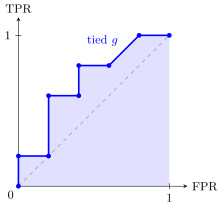
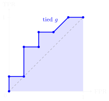
A ROC curve for a sample of five objects of class and five objects of class (schematic). The objects are ordered by decreasing ; an object of class gives a step up of , an object of class a step right of . The slanted segment is objects of different classes with the same value of . The shaded area is AUC ; the diagonal is random guessing.
How is it built? Take all the objects of the sample, compute the values of the discriminant function on them and sort them. Each point on the axis of values of corresponds to one point of the ROC curve. The smallest value is a threshold to the left of all the objects: the whole sample is assigned to class , the false positive rate is maximal, one, and the true positive rate is also one. Then we go along the axis from left to right, and the ROC curve is drawn from right to left, top to bottom. The points, one after another, form a step function: the number of steps along the horizontal axis equals the number of objects of class , and along the vertical each step is a jump over one object of class .
By definition, to compute each point of the ROC curve one would have to compute the numerator and denominator of FPR and TPR, and the amount of computation would be quadratic in the number of objects. Of course nobody does that; it is done exactly as I explained on the plot: going from point to point, we know in which direction to draw the next step of the staircase.
Definition (An algorithm for building the ROC curve efficiently). Input: the sample ; the discriminant function .
Output: the ROC curve , , and the area AUC.
- for all ;
- order by decreasing : ;
- ; ; ; ; ;
- for
- ; ;
- if (taking ), then
- ; ;
- ;
- ; ; .
We order by decreasing values — that is, we go along the curve from the point , with no area yet. We accumulate the increments and for the next step. There is a subtlety here: the values of the discriminant function may coincide on some objects. A step is purely vertical when and , and purely horizontal when . But if there is a run of objects with equal values of , we must accumulate them all and take one step: horizontally by as many as there are objects of class among them, vertically by as many as there are objects of class . Only on reaching a point with a different value of the discriminant function do we build the next step. Sometimes a step turns out to be a trapezoid, and the area of the trapezoid or rectangle is added to the area under the curve; if a step does not go horizontally, the area under it is zero, and nothing is added.
Why did I tell this in such detail? So that you remember one peculiarity. Usually the ROC curve is a staircase, but sometimes you look at a curve that a Python algorithm has built for you and wonder: why are slanted straight lines drawn there? It means that the discriminant function in this classifier has equal values on some objects. This depends strongly on the model: continuous models, like a linear classifier, usually do not behave like this, but with discrete ones, like decision trees, this may well happen.
Remark (If the ROC curve passes below the diagonal). Someone asked: they say the ROC curve should be above the diagonal, but mine first went right along the diagonal and then up. First, the diagonal is the worst classifier there can be: random guessing. If for some reason the ROC curve has passed entirely below the diagonal, the classifier should be flipped, and then it is good. But if part of the way it passes below the diagonal, that is not good. Perhaps most of it is still above, and the AUC is not bad, but there is a zone where the curve is below the diagonal, and on average such a classifier will be not much better than . So it has not been possible to build a good enough model: the problem is hard or the model unsuitable, and further work is needed. One should not put up with it: it is a signal that something is unfinished.
Gradient maximization of AUC
Especially in competitions and in many applied problems the client says: I want an algorithm that maximizes the area under the ROC curve. Why? I want to have a good main model with parameters , and then the freedom to choose a point on the ROC curve to balance type I and type II errors. Fine, we say, since you want to maximize the area under the ROC curve, it would be great to maximize exactly that, explicitly. It turns out to be possible.
Proposition. AUC is the share of correctly ordered pairs :
Here we have summed the vertical values over all the objects of class — simply written the definition of the area under a step curve. If we substitute the formula for TPR here, we are surprised to find that AUC is nothing other than the share of correctly ordered pairs of objects. We take pairs where one object is in class and the other in class ; if the discriminant function gives the correct order relation on these two objects, there is no error on this pair. And it is quite clear what an ideal AUC equal to one is: if in the sorting all the objects of class came first and then all the objects of class , the classifier would be ideal, and the ROC curve would go along the left and top sides of the square. In practice this happens extremely rarely, but an AUC of one is what we strive for.
We have got an unusual quality functional — a sum over pairs of objects — but we know how to work with such things. The dependence on here is piecewise constant. Let us set up something like a margin and approximate the threshold loss by a continuous, or better a smooth, decreasing function of the margin, exactly as in the classification problem. One difference: the margin is now pairwise; it depends on a pair of objects.
Definition (Explicit maximization of the approximated AUC).
where is a decreasing function of the margin, and is a new notion of margin for pairs of objects.
For a linear classifier , ; the stochastic gradient method picks a random pair of objects , , and takes the gradient step
AUC can be maximized explicitly by the stochastic gradient method, very much like what we had in the second lecture. The only difference is that we now choose at random not individual objects but pairs: one object in class , the other in class . We took a pair of objects from different classes and take gradient steps that depend on the margins and on the loss function; there is no other particular difference. This is great: if you have a competition or an applied problem where the client says «I need to optimize the area under the ROC curve», do not use SVM, or logistic regression, or anything else standard. Do it like this — and you explicitly optimize exactly what the client wants. That is the right approach.
The log-likelihood for a probabilistic model
Now imagine a probabilistic classification model — not for nothing did we recall logistic regression in the last lecture; it is just such a model. What if the discriminant function also has a probabilistic meaning, the probability of class ? How should the quality of such a model be evaluated? AUC is categorically unsuitable here. Let us apply an arbitrary monotonically increasing function to . It will turn the probabilities into something completely non-probabilistic — the values may become negative or greater than one — but the ROC curve will stay exactly the same: after all, we build it by sorting the sample by increasing , and a monotonic transformation does not change the order. Hence the conclusion: by the ROC curve we cannot evaluate the quality of the probabilistic model as such, how well the probabilities on the objects are estimated.
Definition (The log-likelihood, log-loss). A probabilistic model of binary classification, : .
The problem: ROC and AUC are invariant under monotonic transformations of the discriminant function .
The log-likelihood criterion (log-loss):
A probabilistic model of multiclass classification: ;
How do we evaluate how well that same logistic regression estimates probabilities? Clearly another criterion is needed, a probabilistic one, and we know it: the log-likelihood, also known as log-loss, the maximum likelihood principle. It is what we optimize, and it is also what should be used to measure the quality of a probabilistic classifier. The generalization to many classes is clear: the probabilistic model is again under the logarithm. These log-likelihoods have another trouble: their values are strange, negative, the larger the better. Models can be compared with each other — which better predicts the class probabilities — but the value of the sum of log-probabilities itself is completely uninterpretable: looking at it, you cannot tell whether it is a lot or a little.
Precision and recall
Another tricky situation arises in information retrieval. Retrieval is also binary classification: when we have a huge number of documents and search them by a query, we classify the documents into two classes, relevant and irrelevant.
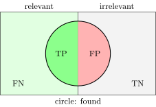
A diagram for precision and recall. The left half is the relevant documents, the right half the irrelevant ones; the circle is what the algorithm found. Precision is the share of green inside the circle; recall is the share of the left half that fell into the circle. Neither depends on TN.
The left half is the relevant objects, the right half the irrelevant ones, the little circle is what our algorithm found. The peculiarity of retrieval is that it does not matter at all how many objects are in the true negative zone, how many irrelevant ones we did not find. So in information retrieval it is customary to use, instead of sensitivity and specificity, two other measures — precision and recall. And note: of the four quantities defined at the start, precision and recall do not depend on TN. It does not matter at all how many irrelevant documents our algorithm did not find — millions or even billions.
Definition (Precision and recall of binary classification). In information retrieval:
Precision is the share of relevant documents among those found; Recall is the share of found documents among the relevant ones.
In medical diagnosis:
Sensitivity is the share of correct positive diagnoses; Specificity is the share of correct negative diagnoses.
It is very easy to remember by looking at the picture: precision is the share of relevant among found, recall the other way round, the share of found among relevant. Recall, by the way, coincides with sensitivity: among the relevant — how many we found. Recall in large-scale search is what is extremely hard to achieve. In the second semester we will have a separate lecture on information retrieval and ranking, and there I will tell you about even more specific measures of search quality. In medical diagnosis it is different: recall and sensitivity coincide, but specificity is not used in search, whereas it is used in medical diagnosis.
The multiclass case: micro- and macro-averaging
Another complication: there are not two classes but more. How do we generalize precision and recall to the multiclass case? For each class one can compute its own TP, FP and FN, and average in two ways.
Definition (Precision and recall of multiclass classification). For each class : are the true positives, the false positives, the false negatives.
Micro-averaging (insensitive to errors on small classes):
Macro-averaging (sensitive to errors on small classes):
With micro-averaging the sums in the denominator are in essence the number of objects of all classes, that is, the unit of analysis is the object. This is bad when the classes are strongly imbalanced. Imagine that one class is 100 times larger than another, and you always assign the small class to the large one. For you this class does not exist at all; the algorithm errs on all its objects, it cannot distinguish this class at all — yet the error will be 1% if you average over objects. So if you want something more or less decent on all classes regardless of their size, measure precision and recall with macro-averaging, averaging over classes.
FPR and TPR on their own, though, are insensitive to class sizes. The ROC curve practically does not change its shape when the classes are rebalanced: increase the number of objects of class a hundredfold — the horizontal steps will become a hundred times narrower, and the curve will stay roughly the same.
ROC and Precision–Recall curves
Can curves be built for precision–recall too? They can; each point again corresponds to a value of the threshold . Let us compare. The ROC curve is a monotonic step function, and the ideal classifier for it is in the upper left corner. With the precision–recall curve one should aim for the upper right corner — precision and recall both good, the higher the better — but it is not monotonic. It has a rather strange shape, and looking at it, it can be hard to say which point is better, this one or that one, and some point is even worse than another by both criteria. The area under it is AUPRC, and the area under the ROC curve in this pair is called AUROC.
Visual clarity is a very important thing that helps to understand different aspects of quality. In classification there are two aspects of quality, tied to type I and type II errors not being the same. And if there are many classes, each class has its own quality estimates. The ROC curve can be built separately for each class and the classes compared with each other: one class may be classified well and another badly. This may say that the class is poorly distinguishable from the others at all, or that there is not enough data on the objects of this class and the model simply does not understand it. A great deal can be extracted from visual analysis based on ROC curves, sensitivity and specificity, or precision and recall.
- Sensitivity and specificity suit problems with imbalanced classes better.
- The log-likelihood (log-loss) suits evaluating the quality of a probabilistic classification model better.
- Precision and recall suit retrieval problems better, when the share of objects of the relevant class is very small.
Aggregate measures:
- AUC suits evaluating quality better when the ratio of error costs is not fixed;
- AUPRC is the area under the precision–recall curve;
- is the -measure, another way of aggregating and ;
- is the -measure: the larger , the more important .
One more thing used in retrieval that I have not yet told you about is the harmonic mean of precision and recall, the -measure. They can be aggregated in different ways, but this simple averaging stuck. And sometimes precision and recall are not equally important to us: in different retrieval problems sometimes precision is more important, sometimes recall. Then a parameter is introduced with which the averaging is done — that is . When people say «the -measure», they usually mean , where , but in some problems, to balance the estimates, is introduced and people speak of the -measure. Such are the subtleties of evaluating classification quality. It would seem nothing could be simpler than evaluating classification quality — but you see how many pitfalls there are here.
Generalization ability and external criteria
Now let us talk in more detail about one aspect we touched on a little in the first lecture: quality outside the training material, the so-called generalization ability, directly tied to the effects of overfitting.
By the way, speaking in the first part of the lecture about classification quality, I never once said on which sample we compute it — on the training or on the test one. It can be computed on both, but on the training one there is no point: an estimate of quality on training is always optimistically biased; that is the effect of overfitting. Of course, all these ROC curves, the areas under them, precision and recall should be computed on the test sample. A very good kind of analysis is to build the ROC curve both on the training and on the test sample and plot them on one graph: it will tell you a lot about how prone the model is to overfitting. It is a very good practice.
The problem of choosing a model and a learning method
Now it does not matter whether we are talking about regression or classification. There is a training sample from which we want to approximate an unknown dependence , and we can build models — and we honestly admit that we have many models, all sorts. We need to choose for the problem the one that is better in the sense of generalization ability.
Definition (The problem of model evaluation and selection). Given: , the training sample; , parametric models, ; , the parameter space of the model ; , learning methods, .
Find: the method with the best generalization ability.
Special cases:
- choosing the best model (model selection);
- choosing a learning method for a given model (in particular, hyperparameter optimization);
- feature selection: the learning method uses only the features .
What does generalization ability refer to at all? To the notion of the learning method, the learning algorithm. It is the map that assigns to a training sample a particular element of the model. A model is a parametric family of functions, and choosing a particular function from it is the work of the learning method. The notion of generalization ability must be applied not to the algorithm built and not to the model of algorithms, but to the learning method, that is, to the way in which we build, optimize, train a particular algorithm from the sample, choosing it from the parametric family.
A special case is the problem of choosing the best model, model selection. For example, we can apply SVM, SVM with a kernel, a neural network, the nearest neighbour method, a decision tree and a few dozen more machine learning methods: how do we choose the best by generalization ability? The next case: the model is fixed, a neural network for example, and we choose the learning method — we optimize hyperparameters. A network has a number of layers and a number of neurons in each layer; these we never train, by backpropagation for example — we train the weights, while the architecture of the network is fixed. Optimizing the architecture, the hyperparameters of the model, is a separate search problem, and the criterion must of course be generalization ability. The third special case, which the third part of the lecture will be about, is feature selection. The model is now the ways of choosing a subset of features. Among the features there may be superfluous ones: uninformative, noisy, dependent on other features, and all this can lead to overfitting. We have already talked about this with linear models as an example. The situation where fewer features are needed to solve a problem than are given at the start is quite typical in machine learning.
Internal and external criteria
Definition (Internal and external criteria of learning quality). is the loss of the model on the object ; is the quality functional of on .
is an internal criterion; it decreases as the model complexity (the number of trainable parameters) grows; a biased estimate of .
is an external criterion; it has a minimum over model complexity; an unbiased estimate of .
Drawback of the hold-out estimate: it depends on the partition .
The quality functional is the mean value of the loss over the sample. An internal criterion is how we evaluate the algorithm built on the training sample itself: we applied the learning method to the sample , got an algorithm and evaluate it on the same sample. This is the very criterion that is optimized during training, and it always gives an optimistically biased estimate of quality. If the losses are to be minimized, the internal criterion may turn out too small, even zero: we are told you have zero errors on the training sample — but that does not mean we have built an ideal classifier; it may be overfitted, everything may be bad with it. To make an unbiased estimate, external criteria are introduced, which evaluate quality outside the training material. For example, on a control sample — such a criterion is called hold-out. There was originally a big sample; we split it somehow into training and test parts, trained on the training , and on the control compute the external quality criterion. What is bad about hold-out? That it depends on the partition: even if it is taken at random, it may introduce a subjective shift into the estimate.
The internal and external criteria against model complexity (slide, the Runge example): the internal one decreases monotonically, the external one has a characteristic minimum.
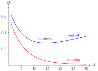
The typical dependence of the internal criterion (the training error, red) and the external one (the control error, blue) on the number of features used (schematic). The internal criterion decreases monotonically; the external one has a characteristic minimum — the optimal complexity.
The main thing about external and internal criteria is how they behave as a function of model complexity. Let us take the number of features as the characteristic of complexity. The internal criterion: the more features, the more degrees of freedom the model has and the more opportunities to fit itself to the training data, and the red curve improves monotonically. But with the external criterion there is, as a rule, trouble: if you overdo the number of features, the control error starts to grow — remember the Runge example. This effect was recognized back in the fifties and sixties by literally every research group that tried to do machine learning, and it turned up in all applied problems. From this the conclusion was drawn that model complexity is evil — more precisely, excessive complexity: excess degrees of freedom, excess parameters begin to fit themselves to the noise, and overfitting arises.
But in the mid-nineties a revolution took place in understanding the role of complexity in machine learning. Boosting was invented, which we will talk about later, and it showed that a model may not overfit as its complexity grows: everything depends very much not only on the number of parameters but also on how the learning method is built. That is, one can work in very complex parametric families and nevertheless not overfit — that is what regularization, dimensionality reduction and many other machine learning techniques are about. If this theory and practice had not been developed for several decades, we would not be seeing today's neural network boom: modern neural networks have millions, billions and already hundreds of billions of parameters — and nevertheless do not overfit. How to achieve this is a very difficult question. The first small step was taken in the mid-nineties, and then theories of overfitting developed; a great deal of work was done on them in the 2000s.
Empirical external criteria: cross-validation
Let us return to the fact that hold-out is bad because it depends on a particular partition. Can this dependence be removed? Of course: take many partitions and average over them.
Definition (Cross-validation (CV)). Averaging over a set of partitions , :
- — a single (random) partition: hold-out;
- is a set of random partitions: the Monte Carlo method;
- — leave-one-out (LOO): each object becomes a control one once;
- , where is a partition into blocks of equal (±1) length, -fold CV: each object takes part in control once;
- , where — partitions into blocks, -fold CV: each object takes part in control exactly times;
- is all partitions: complete cross-validation (CCV).
A special case is hold-out, when a single partition is taken. One can take a random set of partitions — the Monte Carlo method. One can take all partitions — complete cross-validation. Remember, in the lecture on the nearest neighbour method we understood how such functionals can be estimated and even exact formulas derived for them when all partitions are taken; it is one of the approaches of the combinatorial theory of overfitting, but we will not deal with it now. Complete cross-validation is too complicated a thing if there are no theoretical estimates for it, and theoretical estimates are a great rarity: they have been obtained for very few methods; it is a hard combinatorial problem.
What is done in practice? One recipe we already know: leave one out. We train on all the objects but one, compute the loss on that one and average — we have to train many times. Can we save? We can: cross-validation over blocks, -fold cross-validation. We split the sample into blocks, usually , that is, a small number. Each time we train on all the blocks but one, and on the remaining one, using it as the test sample, we check ourselves, and average over all the blocks. We get an unbiased estimate whose training length does not differ very much from the full sample size — we lost, say, one tenth, which is not very bad. And it is computed quite efficiently: we have to train only 10 times, not as many as in leave one out. So such a compromise estimate is very often used in practice.
But it too has a drawback: each object has played the role of a control one exactly once. And if we want to compute, for example, confidence estimates or variances, another standard technique comes to the rescue — -fold cross-validation. We make the partition into blocks times over, each time randomly splitting the sample into blocks differently.
Another important point: the partition into blocks must be random and preferably stratified. Suppose in a classification problem one class is 100 times larger than the other, and we divide the sample into 10 blocks: it may happen that the small class is absent from some blocks altogether. So each class should be split equally into 10 blocks, and then the different classes mixed in each block, and the proportion of classes in each block will be exactly equal to the proportion in the whole sample. This is called stratified partitioning; it is very important when all the blocks need to be representative, that is, to have the same statistical properties with respect to the classes.
And one more interesting point. If we want to estimate confidence intervals, each object must be in control many times, the same number of times . How do we choose ? There is a recommendation: for 95-percent confidence intervals you need 40 measurements, . Why? 40 random points on a segment: the probability that the next one lands to the right of the maximum is about 2.5%, and to the left of the minimum also about 2.5%, 5% in total. That is, if you have made 40 measurements and taken the minimum and the maximum, they give you a five-percent confidence interval for where these values lie at all.
Remark (How many times to train the model). Someone asked: with -fold cross-validation we train the model 10 times, and with — 400 times? Exactly right, 400 times. But I do not insist that you always do 400. is needed when you want to compute a lot of detailed information on the objects: each object has been a test one 40 times, and on it one can estimate the distribution, the confidence interval, the minimum, the maximum, the range. Such detailed analysis is not always needed. If you need only a criterion for selecting models, you can use ordinary -fold cross-validation, and if there is clearly enough of the sample — even hold-out: that is in fact the most common practice. If data are scarce — -fold. And if you also want a detailed analysis on the objects with confidence intervals — .
What does such analysis give? Each object was classified 40 times as a test one, and some number of times it could be assigned to one class and some to the other. If this distribution is close to uniform, the object is uncertain: it is now to the left, now to the right of the separating surface. How many such borderline objects are there? If less than a percent — good. But if 10–20% of the sample, then perhaps the model is sloppy and unstable: you train on different samples, and a large share of the objects falls into the borderline zone, now to the left, now to the right, depending on the composition of the training sample. Most likely the learning method is unstable, and one should work on the regularization or choose another method. From such considerations other quality criteria can also be constructed, for example criteria of classification stability — how concentrated in one class each object's distribution over the classes is. Ideally an object is always assigned to one class, and such objects are the overwhelming majority; how far from ideal your situation is can be measured. It is a costly technique, but it gives much finer information about the quality of models.
And if the data are labelled badly, the labelling is mixed up, there is nothing you can do about that except try to throw such data out; for that there are robust methods insensitive to errors in the data. Another aspect is an unsuccessful model: models may have lower or higher generalization ability, lower or higher stability, and all this can in principle be evaluated with block cross-validation.
Model consistency
Cross-validation is not the end of it: there are many other ideas. One of them is to measure the consistency of models.
Definition (Model consistency). The idea: if the model is right, algorithms tuned on different parts of the data should not contradict each other.
- On one random partition , :
- An analogue of : over partitions , :
Advantage: also suits unsupervised learning.
Drawbacks: the training size is halved; the cost grows by a factor of .
Here too there is a partition of the sample, but now into two equal halves, with stratification of course if it is needed. Let us train the model on one half and on the other: we have trained the model twice on completely different, non-overlapping parts of the sample. The sign that I write, by the way, I have never once said aloud — it is a disjoint union. If there is no overfitting, these two models should, if not coincide, then be very close to each other. Is it true that, training on half the data, we recover the dependence well? If so, we will recover the same dependence from both parts of the data. This is the criterion we call model consistency. An analogue of cross-validation can also be set up, with all the same statistical subtleties: a 95-percent confidence interval will require 40 such partitions, and instead of averaging one can build confidence intervals from the minimum to the maximum. The drawback is that the training size is halved, so this trick works well in problems where the sample is at least twice as large as needed.
Analytic external criteria: regularization
Regularization is in essence also an external criterion. Why? Criteria of the regularization type are an additive term to the internal criterion, a kind of complexity penalty.
Definition (Regularization as an external criterion). A regularizer is an additive term to the internal criterion, usually a complexity penalty for the model :
Linear models: for classification, for regression.
- regularization (ridge regression): ;
- regularization (LASSO): ;
- regularization (AIC, BIC): .
The internal criterion is the one we optimized, and to it we add a penalty, for example for the number of features used. Let us recall what regularization looks like in linear models: the squared norm of the weight vector as the penalty. This corresponds to a Gaussian prior with zero expectation on the model's parameter vector — the probabilistic interpretation; or the interpretation from the point of view of multicollinearity: from the whole infinite set of solutions we choose the most stable one, of minimum norm. regularization is non-smooth, and in a linear model zeroing of coefficients arises, that is, a feature is not used, it is switched off. But this can also be done explicitly — so-called regularization: the penalty is simply the number of features used. In this way we gradually move to feature selection methods, which we will take up in the third part of the lecture.
Definition (Varieties of regularization). The Akaike Information Criterion:
where is an estimate of the error variance and is the subset of features used.
The Bayes Information Criterion:
The Vapnik–Chervonenkis bound (VC-bound):
is the VC dimension, for linear models ; is the significance level, usually .
Where do these words come from — Akaike information criterion, Bayesian information criterion? From different theories of generalization ability, or theories of overfitting. The Akaike criterion was originally built for linear regression models. I am not telling this theory: it is rather old, and much that is better and more interesting has been done since. Here is how the estimate behaves: to the internal criterion we add the number of features used, multiplied by an estimate of the error variance and divided by the sample length. Note: penalties always have a regularization coefficient , which still ought to be chosen based on the balance between the internal criterion and the penalty. But the Akaike criterion says: we have derived from theory what this coefficient should equal; if you can estimate the error variance, here is a way to estimate it. The trouble is that different theories give completely different estimates of the regularization coefficient. The Bayesian information criterion is a somewhat different theory, and the value is different. Hence the conclusion: there is no optimal value. Theories can be built in dozens of different ways, and they will give dozens of different criteria with different regularization. In practice the regularization coefficient has to be chosen empirically, again by some criterion like hold-out or cross-validation, or several external criteria have to be used at once.
For variety, one more regularization, Vapnik–Chervonenkis. I do not tell it in my lecture course, though at one time it was on exactly this that I defended my doctoral dissertation. It involves a characteristic called the Vapnik–Chervonenkis dimension. They are Soviet scientists; they created this theory in the late sixties and early seventies at the Institute of Control Sciences and proposed a Russian term for it — «ёмкость», the capacity of a family of algorithms. For a linear model the capacity simply equals the number of coefficients used, but for more complex models estimating it is a nontrivial business: it is a rather complicated combinatorial quantity. It was later estimated for dozens, if not hundreds, of different families; the problem is hard but quite solvable. In the formula the capacity enters nonlinearly, under a root: the complexity penalty turned out to be proportional to the square root of the number of features, if the model is linear, or of the capacity in the more general case.
This formula is a probabilistic upper bound, strange as it may seem, for hold-out, that is, for the error rate of the trained algorithm on the control sample. In general all these theories proceed from wanting to estimate some external criterion — usually the mean loss on a test or control sample — and a theoretical upper bound is derived for it that depends only on what can be computed by looking at the training sample, on the internal criteria. What is good about this? Unlike hold-out and cross-validation, we sacrifice none of the training sample at all; we spend all of it on training. If we have such a theoretical external criterion — the internal criterion plus a complexity penalty — we can simply apply an optimization method to it and hope that the optimization will give less overfitting. The optimization will still give some overfitting, but this is a way to reduce it, in this case to choose a model of optimal complexity.
Multi-criteria model selection
Model selection can also be multi-criteria: many models can be compared by several criteria at once.
Remark (Multi-criteria model selection). A model slightly suboptimal by both criteria may turn out better than a model optimal by one criterion but strongly suboptimal by the other.
Imagine a plot where two external criteria are plotted along the axes and the points are models. One model is best by one criterion, another by the other, but we will probably choose a compromise one: it is not optimal by either criterion but good by both. In fact the essence of this problem is multi-criteria: if a model can be characterized by different criteria, one should not forget this, should evaluate generalization ability in different ways, and then, preferably visually, choose the model.
Feature selection by an external criterion
We have talked about criteria of classification quality, worked out what external criteria and generalization ability are and how to evaluate them, and now we are armed to take up feature selection. This is the most interesting part of today's lecture.
Definition (The problem of feature selection by an external criterion). is the set of features; is a learning method that uses only the features ; is the chosen external criterion.
is a discrete optimization problem.
This is a model selection problem, a special case of which is called feature selection: the learning method uses only the features from the subset , and we must choose the best learning method among — as many as there are subsets. A wild, astronomical number. If there are few features, 10–20, one can still afford full search, but beyond that, no. This is, first, a problem with a combinatorial explosion, and second, NP-hard: it has been proved that in general the optimal subset of features can be chosen only by full search of variants. We are now going to talk precisely about heuristic methods that avoid full search.
The criterion we choose must be external. Why? Because it has a characteristic shape with a minimum, and our task is to find the minimum point on the lower envelope. Different subsets of features will give a heap of points in this region: along the horizontal axis is the size of the subset, and above each of its values a whole set of models. The optimal subset has to be found.
Full search
The simplest thing one can do here is full search, but cut down somehow. It is cut down because you believe in the existence of a lower envelope that is a unimodal function: it has a minimum.
Definition (The full search algorithm). Input: the set , the external criterion , the parameter .
- initialization: ;
- for , where is the size of the sets:
- — find the best set of size ;
- if , then ; ;
- if , then return .
To build the lower envelope, you go through all values of the size of the feature set — how many features you take — and minimize the external criterion over all subsets of the given size, finding the best set of the given complexity. The vertical set of points is all sets of the same size, and the best model among them is the one with the minimum external criterion. All such lowest points form the lower envelope. All further work, in this algorithm and in all the others, is about how to find this lower envelope faster, computing as few points as possible.
One may believe that the function is unimodal, but that is far from always so: it may be noisy. So having found the best point so far — say at — you do not stop. You increase to five — four is still best; let us take more steps to the right. The parameter , say , is how many more steps you need to take to make sure you have passed through the minimum. The trouble is that on real data the curve may be noisy, and it may seem to you that this is the minimum, while it turns out not global but local — you have to go a little further. «A little» is the parameter , and it will be in all the following methods. You keep track of the with the best model, and if you have taken steps and the model has not improved — stop; larger values of are no longer examined. This is still full search, but somewhat cut down with this heuristic and the confidence that the lower envelope is unimodal or almost unimodal.
Remark (Advantages and drawbacks of full search). Advantages: simple to implement; a guaranteed result; full search is effective when there are few informative features, , and few features in all, .
Drawbacks: in other cases very slow — ; the more variants are searched, the greater the overfitting (especially if the best variants are substantially different and equally bad).
Remedy: heuristic methods of reduced search.
The method is very simple and works quite effectively when there are few features: modern computers allow such a search. But beyond that a combinatorial explosion sets in; variants have to be searched. How are NP-hard problems solved in general? By heuristic methods of reduced search. That is what we will now take up.
Greedy addition
The simplest thing that comes to mind for building the lower envelope quickly but not very accurately is a greedy algorithm.
Definition (The greedy addition algorithm (Add)). Input: the set , the criterion , the parameter .
- initialization: ; ;
- for , where is the size of the sets:
- find the feature most profitable to add: ;
- add this feature to the set: ;
- if , then ; ;
- if , then return .
Advantage: speed , more precisely , instead of .
Drawback: a tendency to include superfluous features in the set.
Remedies: Del, Add-Del, Beam Search.
Again a loop over the set size , and we look for the feature most profitable to add: we see which features were not yet in the set and add one more to the set formed at the previous step. At each step the set grows by exactly one, and greedily each time: we added the feature that gave the maximum gain, but a few steps later it may turn out that this choice was not optimal — and in this algorithm we have no right to look ahead. The rest is as before: we note how many features are optimal, take the extra steps and, if there has been no improvement, return the optimal set — not globally optimal, of course. But we have greatly improved the speed: in the worst case , and in fact times , that is, we will stop much earlier if the optimal number of features is much less than . A very fast method: it cut the cost from to , or even less. But it is greedy, and greed leads to no good: it tends to include superfluous features in the set, and we will not even realise afterwards that they are superfluous.
Alternating addition and deletion
The procedure can be built like this. First we build the envelope by greedily adding features: we went from the point where there are zero features and took extra steps. But now, instead of stopping and saying that the best point found is the answer, we start trying to exclude superfluous features — also greedily: we exclude the feature whose exclusion improves the external criterion most. This is the backward pass. Our swing has begun to swing now forward, now back.
Definition (The alternating addition and deletion algorithm (Add-Del)).
- initialization: ; ; ;
- repeat
- while , add features (Add iterations):
- — the next iteration has begun;
- ; ;
- if , then ; ;
- if , then break the loop;
- while , delete features (Del iterations):
- — the next iteration has begun;
- ; ;
- if , then ; ;
- if , then break the loop;
- while the values of the criterion decrease;
- return .
Advantages: as a rule better than Add and Del separately; fast incremental algorithms are possible, an example being stepwise regression.
Drawback: it works longer and does not guarantee optimality.
We will stop when we see that we have gone forward and back along the same trajectory: first we added certain features, and when we went back, it turns out we are deleting the same features in reverse order. So this will give nothing more, and we stop at a point that may of course differ from the optimal solution, but this is already much better than plain greedy Add and plain greedy Del: Del is the swing going only one way, and if you swing both ways many times, there is hope of finding a much better solution. We have traded speed for quality: Add-Del works more slowly. But back in the seventies insanely efficient procedures were invented for it, in particular for linear regression problems — stepwise regression, with very clever algorithms that allow the solution to be recomputed quickly when a feature is deleted or added. They are used to this day. If you see stepwise regression somewhere, it is a synonym for Add-Del; it is called both ways: stepwise regression, stepwise feature selection methods. It is about adding and deleting one feature at a time.
The blocks of greedy addition and greedy deletion are like twin brothers, and each has the same stopping criterion: extra steps taken. By the way, here can be taken larger, not three but, say, ten, so as to gather extra features and then delete the most superfluous of them optimally. Let the swing swing with a larger amplitude.
Depth-first search and branch and bound
What else can be done? Depth-first search and breadth-first search are two dual strategies very often used for such combinatorial search. Depth-first search is also the branch and bound method. Let me show its essence with an example.
The tree of feature sets in depth-first search, (slide).
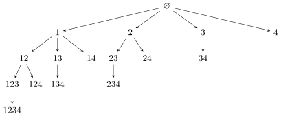
The tree of feature sets for : the features in each set go in strictly increasing order of their numbers, so each subset occurs in the tree exactly once. Depth-first search walks the tree along its branches, breadth-first search by levels.
How do we go through all subsets of four features? A tree of variants: we took feature number one, added feature number two to it, number three, number four; now we go back and say that to «1, 2» we can add four instead of three, and so on. In this way we walk the tree of feature sets depth-first. And the breadth-first walk is by levels: we first built all sets of size one, then all of size two, then three; that is another strategy, which we will consider next.
The technical idea: number the features to avoid repetitions. The tree is unbalanced, and each subset occurs in it only once thanks to the features in each set going in strictly increasing order of their numbers. The sets «2, 3» and «3, 2» are the same subset; the order of the features does not interest us, and there is no need to go through them twice. Depth-first search is a very good way to organize the search so that features are added in strictly increasing order of their numbers.
And where do branches and bounds come in? Building the lower envelope of our set of points, at every moment we have its current approximation, and with iterations it can only move down. Let the best point found so far have size and criterion value . If we have reached a point that is substantially worse and has substantially more features, we will not extend it further, believing that nothing better than the point already found will come of it. This whole range of sets need not even be built: they will most likely be worse than the optimal one found so far.
Definition (Estimating how promising a set is). Let be the value of the criterion on the best set of size among all those examined so far. The set is not extended if there is a such that
and are parameters. The smaller and , the more the search is cut down.
Two parameters arise: — how many extra features we are prepared to take, and — how much more to add to the functional for the set still to be considered possibly promising; if more, it is no longer promising. That is, a set is not extended if we already have a substantially better set with a substantially smaller number of features, and «substantially» is set by these two parameters.
Definition (Depth-first search (DFS, branch and bound)). Input: the set , the criterion , the parameters and .
The procedure extend:
- if there is a : and , then the set is unpromising; exit;
- ;
- for all such that :
- extend.
The main algorithm:
- initialize the array of best criterion values: for all ;
- order the features by decreasing informativeness;
- extend;
- return the for which .
This function is very convenient to make recursive: the procedure «extend» calls itself. If there is a set with a substantially smaller number of features that works substantially better, we say that is unpromising and need not be extended. If it is promising, then for all the features not yet in the set whose number is greater than the largest feature number in the set — this is important: features are added in strictly increasing order of their numbers, to get rid of the superfluous search of sets that differ only in order — we call the procedure «extend» again. Inside it we keep track of the best set, which gave the lowest point on the lower envelope. As iterations go on, the lower envelope gets lower and lower, and thereby we get the ability to cut down the search. At the end this function has to be called with the empty set as input, and the set on which the global minimum of our — approximate, of course — lower envelope was found is returned.
Beam search (GMDH)
Let us move on to the most interesting thing, and to what is used more often in practice: beam search. Do not translate it into Russian as «поиск лучом» or «лучевой поиск»: it is not by a ray but rather by a bundle. This method has a large school: multi-row iterative algorithms, or the group method of data handling (GMDH) of A. G. Ivakhnenko, is in effect beam search in a fairly general statement.
There is a reference there to the philosophical Gabor principle of non-final decisions, which each of us often uses in life: leave yourself as much freedom of choice as possible for making subsequent decisions. The point is to improve the greedy Add algorithm: at each iteration build not one set but a set of sets. In GMDH terminology it is called a row. All the sets of a row have the same size , and their number is bounded above: we consider at most sets at the same time, try to add one more feature to each of them in different ways, and then from all the sets obtained again choose at most . is called the beam width parameter, or the search width.
where is the search width (beam, row) parameter.
Definition (Beam Search). Input: the set , the criterion , the parameters , .
- the first row consists of all sets of length 1: ; ;
- for , where is the size of the sets:
- sort the row by increasing criterion: ;
- if , then — keep the best sets of the row;
- if , then ; ;
- if , then return ;
- generate the next row: .
The pseudocode is very similar to the greedy one. We go over , the number of features in the sets. We sort the row by increasing criterion, and if there are too many sets in the row, we cut it, keeping at most of the best. Then what we always do: look at the best value so far and take at most extra steps. The main thing in this algorithm is how the next row is generated: we take all the sets of the previous row and add to each, one at a time, the features that were not yet in it. In the next row, guaranteed, the sizes of all the sets are again equal, one more than at the previous iteration. So row after row: each row contains sets one feature larger, and from them we choose at most of the very best. Clearly with we get a special case — simply the greedy Add algorithm.
Remark (Additional heuristics).
- Cost: , more precisely .
- Adaptive feature selection: at each step add to the th row only the features with the greatest informativeness .
Clearly, by choosing one can trade off between the cost of the algorithm and the quality of the solution found. Another very interesting idea: as you go, estimate the informativeness of features as the share of cases in which a feature gets into the best sets. Over time statistics will accumulate on how often a feature got into the best ones, and such features can, for example, be taken with higher probability.
Evolutionary algorithms
The next generalization is evolutionary, or genetic, search algorithms. This is very similar to the group method of data handling, only the terminology is different. Feature sets are now called individuals, and individuals are encoded by chromosomes: a subset can be encoded by a binary vector with a one if the feature belongs to the subset. This is a purely terminological difference.
Definition (The evolutionary search algorithm: the idea and terminology). is an individual (in GMDH, a «model»);
is a generation (in GMDH, a «row»);
, is the chromosome encoding .
The binary operation of crossover :
- variant 1: , ;
- variant 2: , ; a «natural» ranking of the features has to be set.
The unary operation of mutation :
- , , where is the mutation probability parameter.
On binary vectors, just as on a genetic code, operations can be defined. Crossover: we took two feature sets, a dad and a mum, and crossed them somehow. This can be done in different ways: take the first part of the features from one parent and the second from the other, or take features with certain probabilities from the dad and the mum. And then mutations can also be arranged. This whole idea of search — pairwise crossover, mutations — was of course spied in living nature, hence «evolutionary algorithms». But there are no mathematical reasons always to cross only two: one can take more, or even generate new sets from a distribution.
Definition (The evolutionary (genetic) algorithm). Input: the set , the criterion , the parameters: , , — the population size, — the number of generations.
- initialize a random population of sets: ; ; ;
- for , where is the generation number:
- ranking of individuals: ;
- if , then selection: ;
- if , then ; ;
- if , then return ;
- generate the th generation by crossovers and mutations: .
In the pseudocode the genetic algorithm differs from the group method of data handling in essentially one line — well, no, in one more place too. The first population is simply random subsets. And unlike the multi-row GMDH algorithm, there is no restriction here that the sets in each row have the same size: in each generation the sizes may differ. And the transition from generation to generation is crossover and mutation: we randomly choose individuals from the previous generation, cross them and mutate them. Otherwise everything is the same as in GMDH.
Remark (Heuristics for controlling the evolution process).
- Increase the probabilities that features pass from the more successful parent to the offspring.
- Accumulate estimates of feature informativeness: the more informative a feature, the higher the probability of including it in a set during mutation.
- Use a set of quality criteria.
- Cross only the best individuals (elitism).
- Carry the best individuals over to the next generation.
- In case of stagnation increase the mutation probability.
- Grow several isolated populations in parallel (the island model of evolution).
I will no longer have time to talk about the heuristics in detail, though modelling evolution on such discrete optimization problems is a very fascinating occupation. After all, what do we do in feature selection? We simply select the best subset by a criterion — for us, an external quality criterion. And there are countless such problems: optimizing a subset of a given finite set by a given criterion. So everything I have told you about here has much wider applicability than feature selection.
Random search with adaptation
And finally, a mega-generalization of evolutionary algorithms: random search with adaptation (RSA). We will generate feature sets simply from some discrete distribution on the set of features. There is no need to look for a dad and a mum — new members of the population should be generated from a distribution.
Definition (Random search with adaptation (RSA)). Input: the set , the criterion , the parameters: , — the population size, — the number of generations.
- initialization: ;
- the population ; ;
- for , where is the generation number:
- ranking of individuals: ;
- if , then selection: ;
- if , then ; ;
- if , then return ;
- increase for the features from the best sets;
- decrease for the features from the worst sets;
- generate the th generation of sets: .
N. G. Zagoruiko, V. N. Elkina, G. S. Lbov. Algorithms for discovering empirical regularities. 1985 (in Russian).
We take the distribution uniform to begin with, because we cannot think of anything better. And then we adapt it: increase the probabilities of the features from the best sets and decrease them for the features from the worst. By what particular formulas I deliberately do not write, because many different formulas have been invented: multiplicative, additive, whatever anyone fancies — dozens of variants, and you can invent more. A generation is produced simply by generating the required number of sets; how many there will be in each population is also a parameter, roughly like the search width in GMDH.
Summary
- These are heuristic methods of discrete optimization.
- must be an external criterion, with a characteristic minimum over model complexity.
- Most heuristics exploit two main ideas: features can be ranked by their usefulness; does not change much with a small change in .
- GMDH, evolutionary algorithms and RSA are very similar — new «symbiotic» metaheuristics can be invented on their basis.
Why do these methods work; why can one get away from full search and make do with reduced search? First, there is hope that features can be ranked by usefulness: among them there are clearly useful and clearly useless ones, and the more contrastingly they are distributed in their roles, in informativeness, the faster we will find the most informative. Second, the hope that the functional does not change much with a small change in the feature set, for example when one feature is added or removed. And last: the three methods I showed at the end — GMDH, evolutionary algorithms and random search with adaptation — are in fact variants of one large family, sometimes called metaheuristics. They are very similar, and new symbiotic methods can be invented on their basis.
No comments yet
Be the first to share your thoughts.