August 30, 2026 · Lecture · LibreTimes
Machine Learning 1. Lecture 7. Generalizations of Linear Models
Contents
- What this lecture is about
- Nonlinear regression
- The Newton–Raphson method
- The Gauss–Newton method
- Logistic regression
- The Newton–Raphson method for logistic regression
- Again a reduction to multiple linear regression
- The IRLS method
- The generalized additive model
- The backfitting method
- The probabilistic meaning of least squares
- The generalized linear model
- The exponential family of distributions
- Examples of distributions from the exponential family
- Maximizing the likelihood for GLM
- Logistic regression as a special case of GLM
- When least squares will not do
- Quantile regression
- Robust loss functions
- Summary
- Seminar
What this lecture is about
Today's lecture continues the previous one. Let us recall what we did last time: we considered the regression problem, the linear regression model and least squares, and within these restrictions learned a lot of interesting things about the solution. Now we begin to drop these restrictions and extend the problem statement to a wider class of problems. Today we will have nonlinear generalizations of regression; situations where linear models can be used but least squares has to be abandoned — that happens too; and non-standard, non-quadratic loss functions. In short, all sorts of generalizations — and the nasty things that happen when we deviate from the classics told in the last lecture.
The lecture will consist of a sequence of relatively separate topics, but they will have a lot in common. One idea will run through the whole lecture: a complex problem can be reduced to an iterative process, at each step of which a simpler problem is solved — as a rule, that very problem of multiple linear regression that we already know how to solve.
Nonlinear regression
Let us start straight with the problem statement. The objects are described by numerical features, that is, they are vectors in ; the answers are real numbers, that is, we recover a numerical dependence of on . An unknown regression dependence, we assume, exists, but we do not know it. Unlike in the last lecture, the regression model is an arbitrary parametric family of functions , nonlinear.
Definition (The nonlinear regression model). Given: a training sample , , ; , is the unknown regression dependence.
Find: the parameters of the regression model .
Criterion — the method of least squares (LSM):
Let us see how far one can get in solving the problem without fixing : let it be some arbitrary nonlinear model. We still want to use least squares — minimize over the sum of squared deviations of the model's answer from the correct value . Last time the model was linear: we differentiated, set the derivative to zero, got a system of equations and studied its properties. That will not work here: in general the problem cannot be solved analytically, only by numerical methods.
We already know one numerical method — the first-order, gradient method, in particular the stochastic gradient method. It can simply be taken and applied to this problem. Full stop, lecture over, let us go home. But no such luck: let us try to apply a second-order method.
The Newton–Raphson method
About Newton methods, in particular the Newton–Raphson method, it is known that they converge much faster, and we can probably profit from that somehow and learn to solve the problem faster than first-order methods allow. Why the formula of the method is exactly so I will not tell: that is from the course on numerical optimization methods.
Definition (The Newton–Raphson method).
- The initial approximation .
- The iterative process
where is the gradient of the functional at the point , a vector in ; is the Hessian of the functional at the point , a matrix in ; is the step size (one can set ).
The main thing is that the iterative process consists of steps in the direction of the antigradient. The gradient points in the direction of fastest increase of the function, and we are solving a minimization problem, so we take it with a minus. But unlike first-order gradient methods, the gradient vector has to be multiplied by the inverse Hessian. The Hessian is the matrix of second partial derivatives: if the gradient is a vector of dimension , equal to the dimension of the parameter vector , then the Hessian is a matrix. The gradient step also appears, but in the Newton–Raphson method it is known that the step can be of the order of one; it can even be set to one. At least some relief: there is no need to choose the step size. On the other hand, technical difficulties arise with the Hessian, and even more with inverting it. Let us gradually work out how to simplify this problem.
First let us write out the components of the gradient vector — the partial derivatives of the functional with respect to . Note: unlike in the stochastic gradient method, I do not get rid of the summation sign; we must honestly carry out the sum over all the objects of the sample; there will be no small steps on each object.
We still keep the function in general form and want to carry it through to the end, to arrive at an iterative process into which any can be substituted to get an optimization algorithm. Let us differentiate once more, with respect to , and get the components of the Hessian:
The expression consists of two terms. With the first we can do nothing, and the second, it is claimed, can be neglected. Why? Let us use a technique physicists love when they meet nonlinear models: linearization. If a function is smooth enough, in the neighbourhood of some point it can be approximately replaced by a linear one. We are at the point , where is the iteration number, and compute the Hessian at this point. Let us, in a small neighbourhood of , replace the nonlinear model by its linear approximation — a Taylor expansion:
The value of the function at the point is a known constant; it can be computed. Then the linear term: is a variable, its fixed value at the point , and the derivative is also taken at a fixed point. The terms of second, third and higher orders we discard. If we substitute this linearization into the second term of the Hessian, the first derivative with respect to a parameter will turn out to be a constant, and the second derivative zero. That is, under linearization the second term vanishes. And the first does not change: the first derivatives at the point of the original function and of its linearization are the same.
The Gauss–Newton method
Let us look carefully at the first term that remains. What does it remind us of? A product of two matrices — the matrices of partial derivatives of the model with respect to all the parameters . Let us move to matrix form.
Definition (The Gauss–Newton method). Matrix notation:
is the matrix of first derivatives;
is the vector of values of .
The formula of the th iteration of the Gauss–Newton method:
where is the solution of the multiple linear regression problem
Nonlinear regression has been reduced to a series of linear regressions. The rate of convergence is that of the Newton–Raphson method, but linear methods can be used for the computation.
The matrix of first derivatives has size : the rows correspond to objects, the columns to parameters. It is like the «objects–features» matrix, only the role of the features is played by the partial derivatives of the model with respect to each of the parameters. is the vector of values of the model on all the objects of the training sample. Let us rewrite the formula of one iteration of the Newton–Raphson method with linearization: the second big term with second derivatives we have discarded, and what remains is in effect the product — it is what we invert; then we multiply by the gradient. We get an expression called the Gauss–Newton method. It is no longer the original Newton–Raphson method: we have replaced the Hessian by an approximation of it. But this method too is known to be of second order, and the rate of convergence has not suffered from linearization.
And now look what we have got. It is the pseudoinverse matrix from the last lecture! There it was built from the «objects–features» matrix as the result of solving the least squares problem for a linear regression model. Let us do some reverse engineering: what linear regression problem have we solved? Clearly, we approximated the vector of differences «model minus correct answers» by a linear combination of the vectors of derivatives of the model with respect to all its parameters. In meaning this also resembles a gradient step: we try to approximate the difference between the model and the vector of correct answers by an optimally chosen sum of the model's derivatives with respect to the parameters. So we have reduced the solution of the nonlinear regression problem to an iterative process, at each step of which a multiple linear regression problem of its own is solved. And that we already know how to solve, and all the methods of the last lecture — the singular value decomposition, principal component analysis if the dimension needs reducing, regularization — fit here and can be applied.
Logistic regression
What we have just considered is nonlinear regression in which least squares remained, and that led us to a second-order method. In the second topic we will keep the model linear but take a linear classification model. The loss function will of course be different: there is no point in using least squares when solving a classification problem. Let us look at logistic regression. We have already talked about first-order methods, about stochastic gradient, and they solve logistic regression well; today we will consider an alternative path — again the Newton–Raphson iterative process.
Definition (The classification problem. Logistic regression). Given: a training sample , , .
Find: a linear model , .
Criterion — the minimum of approximated empirical risk:
where is the logarithmic loss function and is the margin.
A reminder: a two-class classification problem; we denote the classes and . The linear classification model is the sign of a scalar product; is the direction vector of the separating hyperplane, which points towards class , are vectors in , and is a vector of the same dimension. The number of errors on the training sample is written through the notion of the margin: the margin shows the signed distance from the th point of the training sample to the separating surface; if there is no error, the sign is positive, if there is, negative. We replace the threshold loss with an upper bound. Many different such bounds can be made: SVM is one bound, and if we take the smooth function , we get a method called logistic regression. The Newton–Raphson method here is an alternative at least because, first, the loss function is different, and second, we are not putting regularization in here yet, though nothing prevents doing so.
The Newton–Raphson method for logistic regression
Again a second-order optimization method, and again I do not remove the sum, no stochastic gradient: we optimize the sum over all the objects of the sample.
Let us differentiate honestly. The elements of the gradient, the vector of first derivatives :
The elements of the Hessian, the matrix of second derivatives :
where and is the sigmoid function.
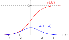
The sigmoid (red), the probability of correctly classifying an object with margin , and the object's weight in an iteration of the Newton–Raphson method (blue). The weight is largest, equal to , at , on the class boundary.
What is ? It is the value of the sigmoid at the margin of the th object. This quantity has a probabilistic meaning, and we will talk about it now, and somewhere in the middle of the lecture I will prove why it is so. Let us look at the Hessian: up to the factor it is the componentwise notation of the product of two matrices . That is, we again recognize the matrix we have to invert: the Hessian again takes on a familiar form.
Again a reduction to multiple linear regression
Let us move to matrix notation. is the «objects–features» matrix: the rows are the objects of the training sample, the columns are the features. From the expressions let us form a diagonal matrix : these values are on the diagonal, all other elements are zero. The factors get in the way in the product of two matrices, and inserting them there amounts to putting the diagonal matrix in the middle, between and .
Proposition. In the matrix notation , :
The step of the Newton–Raphson method coincides with the least squares solution of a linear regression problem with weighted objects and modified answers:
Our aggregate, which gives an iteration of the Newton–Raphson method, is again a construction very similar to the pseudoinverse matrix, only with in the middle. To come to the form , we have to get rid of somehow, and that is not hard: take the root of — a diagonal matrix with the corresponding roots on its diagonal — and multiply by it on the left and on the right. Transforming a little, we will again see that at each iteration we solve a multiple linear regression problem, with the elements of turning out to be the weights of the objects in the least squares statement. The regression model here is linear, and the answers are modified: they are divided by .
An amazing construction. Looking at it, one could try the following: take , approximate them by a linear model and solve the classification problem by ordinary least squares for linear regression. In principle one can, nobody forbids it, though it will not be a very good solution: fitting a linear regression to the numbers and , to class labels. But here we are told that the class labels must be normalized — divided by the probabilities of correct classification.
Remark (Interpretation).
- is the probability of classifying correctly;
- the closer is to the boundary, the larger the weight ;
- the higher the probability of an error, the larger .
Conclusion: at each iteration a more precise tuning on the «hardest» objects takes place.
If an object is classified wrongly, is small, and the modified answer runs off from zero to plus or minus infinity. In this way we tune more strongly to the classification of such an object: if the model errs on the object, we pay more attention to it by increasing its . For classification it does not matter what the absolute value of the model's answer turns out to be: we take its sign, and only the sign interests us. So we can play with the size of the that the regression is tuned to, in order to solve a classification problem.
But that is not all: the modification has also affected the weights of the objects. If is the probability of correct classification, which objects will have the largest weight? Those where . These are the objects on the boundary between the classes, with the most uncertain classification. So, building such a linear regression model, we also pay more attention to the objects lying on the boundary between the classes. We are more attentive to the objects that have turned out to be hard for the current linear classification model at the current iteration. And hardness is of two types: either we err on the object, or the object is borderline and we are unsure of its classification. It is mainly on such objects that we train the model at the next iteration.
Iteration after iteration, a linear regression problem is solved at each step. Hence, by the way, the name: why is logistic regression a regression if it solves a classification problem? That is why. The second-order method I have told you about is the textbook, classical method for solving the logistic regression problem. And it is also a regression because it predicts the probabilities of objects belonging to a class, and a probability is no longer a discrete quantity but a continuous one. This too brings logistic regression closer to regression, although a classification problem is being solved.
The IRLS method
Let us put everything together and write the pseudocode of the iterative process, so as not to get lost in the intermediate computations.
Definition (Iteratively reweighted least squares (IRLS)). Input: , — the «objects–features» matrix and the vector of answers.
Output: — the vector of coefficients of the linear combination.
- — the zeroth approximation, ordinary least squares;
- for
- for all ;
- for all ;
- ;
- for all ;
- choose the gradient step ;
- ;
- if the have changed little, exit the loop.
The zeroth approximation is that very unfortunate way of using regression for classification: we took our and substituted them into the ordinary solution of the least squares problem for multiple linear regression, with the pseudoinverse matrix from the last lecture. It is a rough solution of the classification problem by regression, but it will do as a zeroth approximation. Then at each iteration, for the current approximation of the vector , we compute — the probabilities of correctly classifying the objects of the training sample — compute the diagonal matrix, multiply the features by it on the left and reweight the answers, multiplying them by a factor that depends only on . So we have reweighted both the objects and the answers. The gradient step in the Newton–Raphson method can be set to one, or it can be finely tuned at each iteration if one wishes. What happens at the eighth step is the solution of a multiple linear regression problem. We have reduced a new, harder problem to the successive solution of problems we already know how to solve, as was done in the last lecture.
Remark (Why there is a root in). Someone asked: why is equal to multiplied by a root, when earlier we divided by ? I am not deceiving you here, but I hid a few lines of calculation. In the step there was ; to get we multiply on the left by , that is, by the roots of . But on the right there is also , and it too has to be made into , and for that the vector on the right has to be multiplied and divided by . The ratio multiplied by gives the root:
The generalized additive model
The third topic falls somewhat out of the main narrative, but it is an important thing, and it had to be told somewhere; now is the best moment. We want to generalize the linear regression problem, but in a limited version: not to introduce an arbitrary nonlinear dependence on , but to say that all we lack for a linear model is to transform each individual feature a little — to bring it into a form in which a linear model can be built over the transformed features.
The best example is the applied problem I gave in the first lecture: predicting real estate prices. The price of a flat in Moscow is made up of many factors: floor area, the number of rooms, a balcony, and God knows what else. Some features are numerical, others binary, like having a balcony. But what about a feature such as the distance to the metro? Intuition suggests that the greater the distance to the metro, the smaller the contribution to the price: the closer to the metro, the higher the price of the flat. One could put this distance into a linear regression, and probably a negative coefficient would come out. But are we sure that the distance to the metro makes a literally additive, linear contribution? Rather not: it should be some decreasing function, and we would like to find out what it looks like — to train it too, tune it, optimize it. There are quite a lot of such problems: one wants first to perform a separate learnable nonlinear transformation on each feature separately, and then build a linear regression model over the transformed features.
Definition (The generalized additive model (GAM)). Find: nonlinear transformations of the features (in particular, with this is a linear model):
Criterion — the method of least squares.
Idea 1: refine the in turn on the sample :
Idea 2: gradually decrease for the smoothness regularizer
Use splines or kernel smoothing as the .
The model is the sum over all the features of their transformations. A transformation may also be linear — simply multiplying the feature by the coefficient , and then it is a special case, the ordinary linear regression model. But we want to allow nonlinear transformations of individual features, and we need to train the functions — functions of a scalar argument with some parameter. Let us write least squares for such a model and train the in turn: training one, we fix all the others; having trained it, we take another feature and train its , and so on until the process converges to something. The fixed other functions form a construction we will call , and we get the problem of training a one-dimensional regression model, no longer on but on the differences between and the sum of all the other, fixed transformations of the features.
Regularization can also be added here. We may assume that the function transforming the feature is smooth enough, that is, does not differ too much from a linear one. That very decreasing function that converts the distance to the metro into a unit price — how much the price of a flat decreases with every hundred metres from the metro — is monotonically decreasing, probably not too complicated and not too different from a linear dependence. We do not mean it to have any humps, ridges or sinusoids. How do we introduce such an additional constraint — that we want a function as simple as possible in the sense of smoothness? An example is the regularizer that is the integral of the squared second derivative: for a linear function the second derivative is zero, and the integral is zero; a small non-smoothness, a small nonlinearity lead to small values of this penalty term.
There are methods that directly solve the one-dimensional problem with such a regularizer, splines for example. One can also do it differently — by kernel smoothing with the Nadaraya–Watson formula. Choosing the smoothing window width there is roughly the same as choosing the regularization coefficient : the larger , the smoother the function we get, and the wider the window, the smoother the function we get. So the one-dimensional problem is fairly easy to solve. Moreover, the one-dimensional problem is easy to visualize: one can plot the approximation of the one-dimensional dependence of on and see whether the chosen function really describes it well.
The backfitting method
We get a method into which visual quality control of the solution can be inserted at each step. It is called backfitting, and it is rather old: Hastie and Tibshirani invented it back in 1986. It is good precisely in problems like predicting real estate prices, where one wants to check with one's eyes how meaningful the nonlinear transformations of each feature come out. For the distance to the metro you expect to get some nontrivial — a monotonically decreasing function, and it is interesting to look at it. But for the floor area of the flat you hardly expect any clever nonlinear transformation and may well leave the linear dependence as it is.
Definition (The backfitting method (Hastie, Tibshirani, 1986)). Input: , — the «objects–features» matrix and the vector of answers.
Output: — learnable transformations of the features.
- initial approximation: the solution of the multiple linear regression problem with the features ; , ;
- repeat
- for
- , ;
- ;
- decrease the regularization coefficient ;
- while and/or decrease noticeably.
Look how interesting. In the previous two topics we also built an iterative process, and at each iteration the nonlinear problem was replaced by the classical linear regression problem. Here too a replacement takes place, but a different one: solving the problem at each iteration reduces to solving a one-dimensional nonlinear regression. There we replaced a nonlinear model by a linear one at each iteration; here we replace a multidimensional problem by a one-dimensional one.
Let us go through the code. The initial approximation: again one can solve the multiple linear regression problem and say that is simply multiplying by the coefficient . This is the first approximation; we will substitute it when computing — what the one-dimensional model is tuned to for each feature; the target for us is now , but only at this iteration; at each iteration it is different. I write the one-dimensional problem in general form, though it is implied that you choose yourselves: splines, Nadaraya–Watson kernel smoothing, some other approximation — anything. But in any of these methods a parameter that has to be optimized will appear one way or another. With too strong smoothing you will get a linear model, and there will be no nonlinearity in the feature transformation. With too weak regularization you may overfit: zero errors on the objects of the training sample, but a too complex, rapidly oscillating function . So the regularization has to be chosen by looking at how the function behaves and how well it passes through the sample points. In this way, step by step, by successively complicating the solution — gradually decreasing — we build the model.
Remark (Where to read). Someone asked where to read about splines. That is thousands of publications. One of the best textbooks, in my view, is The Elements of Statistical Learning; among its authors are Hastie and Tibshirani, the authors of the backfitting method. It has gone through many editions: the authors try to put the latest methods and trends into the book, the book swells with each edition, but it is gradually ageing, of course. There is something about splines in it. In general, spline theory developed in the sixties and seventies, and I believe earlier; it is a very well worked-out theory, with many books and textbooks on function approximation.
The probabilistic meaning of least squares
Now the most important part of today's lecture, in my view — generalized linear models. But first let us sort out the names. The backfitting method is a generalized additive model; do not confuse it with the generalized linear model, which we are about to discuss. The names are similar; the meaning is completely different. Let us start with the close link between least squares and maximum likelihood and understand what probabilistic meaning least squares carries. It is nontrivial.
Definition (The probabilistic statement of the regression problem). Given: a sample , , .
Find: the parameter of a regression model with Gaussian noise:
An equivalent notation: , .
We will build a model of the data, assuming that the are predicted by our model up to the noise . This noise is the residual between the model and the true unknown target dependence. We will assume that the model is so good that the residuals have certain probabilistic properties: they can be considered normally distributed with zero expectation. Zero expectation is the assumption that the model is unbiased: it approximates the target dependence so that the errors are now positive, now negative, with no systematic bias. And another assumption is that we know the variances or can estimate them. And in general the variances on different objects may differ: on some object we can predict more accurately, and on some the noise variance is larger, and we cannot claim high prediction accuracy there. Sometimes a stricter assumption is made, that all the variances are equal — this is called the homoscedasticity assumption for the residuals. We are now in a more general statement: unknown and different variances are assigned to the residuals .
An equivalent notation: the have a normal distribution with some expectations and unknown variances , and the expectation of is our model. Such is the probabilistic view of regression: regression describes the expectations of the , up to noise, and about the distribution of this noise we assume Gaussianity.
Let us apply maximum likelihood, since we have ended up in a probabilistic statement. The random variables here are the ; let us write out their joint density: they are distributed with zero expectation and variances .
Proposition. The maximum likelihood criterion is equivalent to least squares:
Where are the parameters here? : on the one hand the are random variables, and on the other they are functions of , and the problem can be solved as an optimization problem over . The most interesting thing: if we maximize the log-likelihood, we get a sum of logarithms, the logarithm and the exponential destroy each other, and we unexpectedly see that the maximum likelihood principle is equivalent to least squares. is the square of the difference between the model's answer and . This is least squares, with a small generalization: we also ended up with weights of the objects.
And this too is an interesting insight: it turns out that in least squares the weight of an object is nothing other than one divided by the noise variance on this object. The larger the noise, the smaller the weight: if we understand that a good prediction is impossible on some objects, there is a large noise variance there — the weight of such an object in the least squares criterion should be reduced proportionally. So least squares is not taken out of thin air: behind it stands the implicit assumption that our model is so good that it is unbiased, has zero expected errors, and that the noise is Gaussian.
A question arises: if for some reason we are not sure that the errors are Gaussian, do we then have no right to use least squares? Generally speaking, yes: something else has to be used, having made another, more plausible assumption about the form of the error distribution. And one more consideration: if we predict an integer quantity rather than a real-valued one, can we expect the errors to be Gaussian? Most likely not, and we should understand what error distribution would be more adequate in this case. What should be used instead of least squares if the are not Gaussian, in particular if they are discrete-valued?
The generalized linear model
Let us generalize least squares so as to approximate dependences by models for which we are not sure that the errors are Gaussian and can write out some alternative formula for the error distribution. Such a generalization is called the generalized linear model: we do want to stay within linear models.
Let us start again from the normal linear model for the expectation: we assume that the are normally distributed and their expectation is described by a linear model. This is the standard statement, closely tied to least squares. Now we generalize: instead of the Gaussian distribution we take a very wide class of distributions called the exponential family. But everything has to be paid for. For widening the class of distributions we will pay with the fact that the parameter , which we will model linearly, is now not equal to the expectation of but is tied to it through a known function — the link function.
Definition (The generalized linear model (GLM)). Given: a sample , , .
Find: the parameter of the generalized linear model (GLM):
Instead of the assumption that the are Gaussian, is now introduced — the exponential family of distributions with the parameter , the scale parameter and the function parameters , :
Criterion of maximum likelihood:
The exponential family of distributions
The exponential family is specified up to two parameters, and , called the location and the dispersion respectively. They are some analogues of the expectation and the variance, but they are exactly these only for the Gaussian distribution; since not exactly, they have other names. And the exponential family is also specified by two functional parameters: the function and the function .
Look what a formula, from who knows where. The main thing is that it is the exponential of something, and inside it there is a form linear in : is multiplied by ; the function depends on but not on or ; and the function does not depend on . A kind of decomposition has happened: the exponential of a sum is a product of exponentials, and the distribution can be represented as a product of two functions, one of which does not depend on , and the other depends on only linearly. I will now give examples, and it will turn out that very many well-known distributions are special cases of the exponential family.
Theorem. The expectation and variance of a random variable :
is the monotonic link function.
What is important for us to know about the exponential family? First, for a random variable generated by the exponential family one can compute the expectation and the variance. I omit the calculation: it is not hard; the corresponding integral has to be computed. It turns out that the expectation is , the derivative of the function of the scalar parameter . Hence is expressed as a function of the expectation: the inverse function of the derivative. We conclude that must be monotonic so that its inverse can be taken. This is the link function, linking the expectation with the parameter . And we declared from the start to be modelled by our linear model — not the expectation, as before in the simple case of least squares. For the generalization we have to pay with the appearance of the function . But we know how to compute it: as soon as a particular distribution from the exponential family is written out, we know the function , can differentiate it and find the inverse. That will be the link function. So it does not create any special technical difficulties for us.
Proposition. The normal linear model is a special case of GLM:
Examples of distributions from the exponential family
Let us consider four examples.
Example (The normal (Gaussian) distribution,).
What has to be done to get everything under the exponential in the normal distribution? Take the logarithm of the normalizing factor and bring it inside, and expand the squared difference and regroup the brackets a little. is the identity function, and such a miracle happens only in the Gaussian distribution as a special case of the exponential family. And here really does turn out to equal the variance — hence the name «dispersion parameter»: in the Gaussian case it equals the variance, and for other distributions it may be something else.
Example (The Bernoulli distribution,).
Why is the Bernoulli distribution interesting? Because it is the two-class classification problem. When the residuals are normal, it is a regression problem, where we are entitled to apply least squares. But if we are solving a classification problem, we are not entitled to apply least squares: we cannot assume that the are Gaussian. They are distributed by Bernoulli: one class has probability , the other , that is, with probability and with probability ; the formula writes the same thing as a product. Bringing this notation to the exponential form is very easy: we artificially introduce an exponential — first put the expression under a logarithm, then take its exponential — and indeed turns out to be multiplied by something depending only on the expectation. That is , and can be expressed through it. There is no dispersion parameter here; it equals one.
Example (The binomial distribution,).
The binomial distribution is the number of successes in a Bernoulli scheme. It arises in problems where we want to approximate the probability of a discrete event, knowing that the maximum number of times the event could have happened is known and equals . On each object there is some counter: the maximum number of times is known to us, and we observed the event some number of times, and these data are the to be predicted: how many times the event will happen on the given object. Since we predict an integer quantity — the number of successes in a Bernoulli scheme — it has a known distribution, the binomial. At first sight the formula even has the combinatorial coefficients , but it is easy to show that this too is an exponential family: we put everything under the exponential and are surprised to find a linear term with exactly the same formula as for the Bernoulli distribution. Well, not quite the same: there it was one, and here it is a known integer . The dispersion parameter does not need estimating either.
Example (The Poisson distribution,).
The Poisson distribution is a limiting special case of the previous one: we do not know how many times the event could have happened, but we predict some integer quantity. For example, the number of clicks on an advertising banner: CTR (click-through rate) in many problems of internet advertising, in problems related to recommender systems and in many other places, an integer quantity arises, and it is unknown what its upper limit is. Unlike the binomial distribution, where the maximum number of successes is known in advance, here it is unknown how many times users could have clicked, yet one wants to predict the probability of a click. Then the Poisson distribution may be more appropriate. Again we put everything under the exponential, find multiplied by something depending only on the expectation — and that gives the link function of the expectation with , which we approximate by a linear model. And again equals one. That is, in three discrete distributions very often needed in practice, the dispersion parameter does not need estimating, and that is a pleasant simplification.
I have shown four examples of how one proves that a known distribution is a special case of the exponential family: put everything under the exponential, collect like terms, and it becomes obvious what the functions and equal. But this cannot be done with every distribution.
Remark (Which distributions belong to the exponential family). Examples: the normal (Gaussian); the Poisson distribution; the binomial and multinomial; the geometric; the distribution; the beta distribution; the gamma distribution; the Dirichlet distribution; the Laplace distribution with a fixed expectation.
Counterexamples (non-exponential distributions): Student's distribution, Cauchy, the hypergeometric.
The list of useful distributions that are not exponential is in fact much longer, and it is rather an exception for a distribution to be exponential. But in practice it is exponential distributions that arise very often. Once again: this is about the distribution of the quantity that we are going to predict. If some theory tells us that the predicted quantity is distributed according to some distribution — , Dirichlet, beta, gamma, Poisson and so on — this theoretical knowledge should be treated carefully. Since we are predicting a quantity that is not Gaussian, we have no right to use least squares: we must use maximum likelihood explicitly, modelling the distribution of the .
Maximizing the likelihood for GLM
Let us do this in the general case, for an arbitrary distribution from the exponential family, and see along the way why it has exactly this form.
where depends linearly on : .
We substitute the formula of the exponential distribution and take the logarithm at once: the logarithm and the exponential destroy each other. But I immediately used one more trick. The function depends on and ; if is a constant, one for example, then can be thrown out; it will not depend on the parameters. Moreover, if we assume homoscedasticity — the dispersions are the same for all objects, that is, there is no reason in the model to think that on some objects the errors will be much larger than on others — the formula simplifies: only the first terms remain, and the terms with go away, because they depend neither on the model parameters nor on the objects of the sample. This cannot always be done; look carefully: if this term does not drop out, it has to be taken into account carefully. And once again let me remind you where is here: is the linear model itself, the sum of all the features of the object with the weights , so the maximization is over , on which depends.
A good, pleasant functional, and it has to be optimized. We have already done this trick twice today; let us do it a third time — the Newton–Raphson method:
You can already guess what will happen next. We honestly differentiate with respect to and .
The components of the gradient vector :
The components of the Hessian :
And again we will have to invert a matrix very similar to the product , only a factor has crept in that depends on the object but not on the features and . Again this will be a diagonal matrix inserted between and , and we will probably now see iteratively reweighted least squares again.
Proposition. Matrix notation: is the «objects–features» matrix;
, are the weights of the objects, ;
, is the modified vector of answers.
Then the Newton–Raphson method again leads to IRLS:
This coincides with the least squares solution of a linear regression problem with weighted objects and modified answers:
From the «objects–features» matrix we form a new, reweighted one, and we reweight the answers: subtract the expectation and divide by something like the spread — the root of the variance ; clearly this is the modified vector of answers. And the Newton–Raphson method again leads to iterative reweighting, that is, to solving a linear regression problem. I will not interpret it further: that is somewhat more complicated than for logistic regression, but the meaning is roughly the same. Again we have reduced the problem to a series of multiple linear regression problems. Let us write the pseudocode once more, now for the more general statement.
Definition (IRLS for GLM). Input: , — the «objects–features» matrix and the vector of answers.
Output: — the vector of coefficients of the linear combination.
- — the zeroth approximation, ordinary least squares;
- for
- for all ;
- for all ;
- ;
- for all ;
- choose the gradient step ;
- ;
- if the have changed little, exit the loop.
The essence of the process is the same. The zeroth approximation is ordinary least squares, as if it could be applied; it will do. Then we compute the linear model, the weights, reweight; the gradient step can be set to one or chosen. At the eighth step is the pseudoinverse matrix, that is, the solution of the multiple linear regression problem for the answers and the «objects–features» matrix transformed by these formulas. That is all — very similar to what we got for logistic regression. And this is no accident: substituting and of the Bernoulli distribution, we get exactly IRLS for logistic regression. Logistic regression is a special case of the generalized linear model.
Logistic regression as a special case of GLM
Let us consider logistic regression as a special case of GLM and understand the main thing: where the sigmoid function in logistic regression comes from, and where the probabilistic interpretation comes from. It turns out that the only source of this is the probabilistic assumption that we predict distributed by Bernoulli. The essence of this assumption is just one thing: we assumed that for each object there exists a probability of class . We made no other probabilistic assumptions. And this probability is also the parameter of the Bernoulli distribution and also the expectation. Everything else follows automatically from the general theory.
Definition (Two-class logistic regression). The Bernoulli distribution, : ;
Given: a sample , , .
Find: the probabilistic model .
Criterion — the maximum of the log-likelihood (log-loss):
A convenient recoding: :
is our linear model, is the expectation, that is, the probability of class for the th object. The link between them is the link function; if we write the inverse function — wow, it is the sigmoid function! So that is where it came from. And if we write the maximum likelihood functional, that very logarithmic loss function pops out — a direct consequence of the link function, that is, of a single probabilistic assumption: has a probability of belonging to a class. From it both the sigmoid and the logarithmic loss in the functional equivalent to maximum likelihood popped out at once. That is, these are not heuristics but consequences of the probabilistic assumption that a probability of class exists for each object of the training sample. Look what a harmless probabilistic assumption we made, and what interesting consequences we got in the form of a particular loss function. This, in my view, is a little bit fantastic, a very beautiful mathematical consequence. And at last you understand where logistic regression came from.
Let us do the calculation I described in words. Here we have to do a little alchemy with the coding of the classes: in the Bernoulli distribution , while in linear models we are used to denoting the classes and . One can be recoded into the other, for example, by the formula . For the object the probability of belonging to class is the expectation, through the link function it is . And the probability of class is , thanks to the property of the sigmoid function . From these two equalities we conclude that the probability of for is the sigmoid of the margin: . So that is what it is: the margin, written through taking the values .
The maximum of likelihood — which is also the minimum of the log-loss criterion — can be written in two equivalent ways. On the one hand, it is the sum over all the objects of the sample of the logarithms of the probability of the class for the object , written through the Bernoulli distribution. This form of the criterion is often called log-loss, and in very many places, in many binary classification problems, everything starts by writing out this criterion. The other way of writing is through the logarithmic loss of the margin. One can write it either way when one meets a probabilistic statement of the problem. This, in my view, is the central insight of today's lecture about logistic regression; now one can say that you know the main things about it. And the optimization here can be done by the second-order method, IRLS, or by the stochastic gradient method I have already shown you.
From just two assumptions:
- the are Bernoulli random variables with ;
- the parameter is linked to the linear model: ,
follow the most important properties of logistic regression:
- the logarithmic loss function ;
- the sigmoid link function ;
- the link of the linear model with the odds ratio:
One more small addition: the value the linear model gives on an object also has an interesting probabilistic meaning. It is , which is also , that is, the logarithm of the odds ratio — the logarithm of the ratio of the probability of the object being in class to the probability of it being in the other class. It turns out that the numerical value of the scalar product is not only the distance from the object to the separating hyperplane but also the logarithm of the odds ratio. A very interesting probabilistic interpretation of the linear model. And all this, let me remind you, follows from just a single assumption: the classes have a Bernoulli distribution, and the Bernoulli distribution has a single parameter, which is also the expectation, the probability of class .
When least squares will not do
The last topic is other cases where we have no right to use least squares, although we would very much like to: it is such a developed method, all the ready numerical methods exist for it.
Let us start with the fact that we do not always want to minimize squared errors. Least squares has a solution for the case where the model is a constant; we have already discussed it, including when deriving the Nadaraya–Watson formula. The model is just a scalar parameter , with no dependence on ; differentiating with respect to and setting the derivative to zero, we immediately get that is the mean value of on the objects of the training sample. And if we want to minimize not the sum of squared deviations but the sum of absolute values? Solving the analogous problem for a constant, we will see that the solution is the median of the , not the arithmetic mean.
Example (The mean, the median and the quantile as solutions of problems with a constant model). The arithmetic mean (unstable to large outliers):
Let be the order statistics, the values in increasing order. Ways of averaging that are robust to outliers:
- the median:
- the -quantile:
What is good about the median? It is much more robust to outliers. If a very large error has crept in among the — for example, instead of something a million times larger was taken — the arithmetic mean will jerk very strongly in that direction: it is sensitive to large errors in measuring the . But the median does not care; it will not jerk anywhere: the anomalously large value will end up last in the order statistics, and in the middle, most likely, the same value or its neighbour, very close to it, will remain. Hence the property: the method of least absolute values, with such a loss function, is preferable in problems where extremely large outliers are expected. But what does that mean? That the distribution of the is not Gaussian. Assuming the presence of outliers, we assume the Laplace distribution — with heavy tails, also exponential, but depending on the absolute value of the error rather than its square.
Quantile regression
A generalization: what if the loss function is not just the absolute value but a skewed absolute value, and the penalties for positive errors are smaller than the penalties for negative ones?
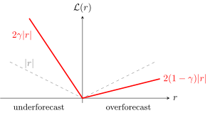
The skewed absolute value of the error (red, ) beside the ordinary absolute value (grey): an underforecast is penalized more than an overforecast. For a constant model the solution is the -quantile of the answers, not the median.
For example, in the problem of forecasting sales volumes. If we made an underforecast — the goods were not delivered — we created a shortage and did not get the trade markup: those are large losses. And if an overforecast — too much was delivered, funds were frozen, the goods sat on the shelf but still sell — the loss is smaller. Such situations arise in different applied problems. If we want to measure losses literally in roubles, they will be a linear, not a quadratic, function of the forecast errors: a square of roubles has no economic meaning, accountants tell us. Why use least squares in such problems? Skewed absolute values should be used.
What will the constant solution be? Instead of the median a quantile of the distribution will appear — hence the name quantile regression. If we take the order statistics of the values and in them take not the middle value but the th, where is computed from the slopes of the two branches of the loss function, then this solution is optimal. For a primitive, constant model the solution of quantile regression is a quantile, that is, an element of the order statistics of the values of . The more heavily an underforecast is penalized, the higher up the order statistics the optimal forecast.
And if the regression model is linear, quantile regression is easily written out so that it reduces to a linear programming problem — minimizing a linear criterion under linear equality and inequality constraints. For example, like this: represent the residual as the difference of two non-negative variables, the positive and negative parts, as we did for LASSO,
The problem of forecasting sales volumes is in practice quite often solved precisely with quantile regression and linear programming. It can be even trickier; I believe I showed this in the first lecture when telling about forecasting sales volumes: the loss function may be piecewise linear made not of two pieces but, for example, of five. With different sizes of overforecast the loss factors change: the more we overbought, the more new factors come into play, and the losses begin to grow with a different coefficient of proportionality. And the large losses from an underforecast are tied to the loss of the trade markup and of customer loyalty.
Robust loss functions
There are also loss functions invented in order to ignore large errors in measuring the . For example, instead of the quadratic loss we want to take a function with horizontal asymptotes. Many such functions can be invented.
Definition (Loss functions for robust regression). The loss is a function of the error . The quadratic loss is not robust.
Robust loss functions with a parameter :
- — piecewise linear (Least Absolute Regression);
- — piecewise linear (SVM Regression);
- — Meshalkin's;
- — Huber's;
- — Tukey's.
Barron's family of functions with a parameter :
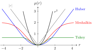
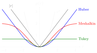
The quadratic loss (black) and robust ones: the absolute value (grey), Huber's (blue), Meshalkin's (red), Tukey's (green), all with . The branches of the robust functions grow linearly or approach a horizontal asymptote, so large errors hardly affect the tuning of the model.
Here, as an example, is Meshalkin's function. The problem with such a loss function is also not least squares; it too is, one could say, maximization of likelihood, and one can even write out the error distribution — it will of course be not Gaussian but some other. But one can also not bother with probabilistic interpretations and simply say: we took such a loss function, and we solve the problem by the same Newton–Raphson method. I will not write it out for you a fourth time.
There is also Barron's parametric family of loss functions: by changing the parameter one can get both the parabolic loss (at the value 2) and loss functions with horizontal asymptotes. Within one parametrization one can change the model's attitude to noise in measuring the . In general robust regression is a big research topic; thick books on robust regression have been written, and I have a separate lecture on robust models; for now only a spoiler, and the lecture will be in another semester. Many functions have been invented — Meshalkin's, Huber's, Tukey's, Andrews' and many other surnames — and most of them have the property that their branches, unlike the parabola, are either horizontal or have a linear order of growth. That is, they are more tolerant of large errors and, when the model is tuned, simply pay no attention to them.
SVM regression I have also already told you about in the lecture on SVM: it too is an example where in a regression problem the classical loss function was replaced by a piecewise linear one and all the properties of the SVM method were obtained — support objects and a quadratic programming problem; everything is very similar to SVM for classification. So we have run through the cases where something other than least squares has to be used, and as a rule this follows from the understanding that our errors are not Gaussian.
Summary
We have come to the point where an iterative process has appeared three times, no, even four times: in nonlinear regression, in logistic regression, in the generalized linear model and in problems with non-quadratic loss functions. That is today's main message: complex problems can be reduced to an iterative process — to a series of solutions of simpler linear problems that we already know how to solve.
- Logistic regression is not regression but classification; the Newton–Raphson method leads to IRLS.
- The generalized linear model (GLM) powerfully generalizes ordinary and logistic regression; the Newton–Raphson method leads to IRLS.
- The generalized additive model (GAM, backfitting) reduces to a series of one-dimensional smoothings.
- The probabilistic meaning of the loss function: it is of the probabilistic model of the data.
Today's main topic is still the generalized linear model. It is applied in very many places, both in machine learning theory and in practice, and is well studied; I gave you a simplified account. Thick surveys and books have been written about it, but for a general understanding of what was today, this is enough for you.
No comments yet
Be the first to share your thoughts.