August 30, 2026 · Lecture · LibreTimes
Machine Learning 1. Lecture 6. Linear Regression Models
Contents
- What this lecture is about
- Multiple linear regression
- The normal system of equations
- The geometric meaning of least squares
- The solution through the singular value decomposition
- Multicollinearity and the condition number
- Ridge regression
- Choosing the regularization parameter
- Regularization reduces the «effective dimension»
- LASSO and non-smooth regularizers
- A geometric interpretation of feature selection
- Non-smooth regularizers for selecting and grouping features
- Principal component analysis
- The link with the singular value decomposition
- The effective dimension of a sample
- Principal component analysis in linear regression
- The spectral method of least squares
- Low-rank decompositions: what comes next
- Summary
- Seminar
What this lecture is about
We continue studying linear models, and today it is about regression and the method of least squares, which, generally speaking, we have been talking about since the first lecture. The plan is this. We start with the classic, textbook problem of multiple linear regression and see how it is solved with the singular value decomposition. We talk about regularization again. Then about principal component analysis: it too is an application of least squares, but to a quite different problem — not building a predictive model but transforming the feature space. And at the end we will bring everything together, and I will show a very unexpected insight about least squares that is rarely written or talked about.
Multiple linear regression
Let us start with the familiar notation.
Definition (The optimization statement of the learning problem). is the space of objects; the set of answers (predictions, estimates, forecasts); the unknown dependence (target function).
Given: , the training sample; , a parametric model of the dependence.
Find: , the parameter vector of the model.
Criterion — the minimum of regularized empirical risk:
where is the loss function and the regularizer with regularization coefficient .
Today the answers are real numbers, . In least squares the difference is the model's error on the object; for mathematical convenience we square it and sum over all the objects of the training sample. We could also assign weights to the objects — by default all objects are equally important — and we have already seen one trick with weights: the Nadaraya–Watson formula was also least squares, and the game there was precisely with the weights. Today we leave them alone; the weights are ones. And a terminological detail: the value of the functional at the minimum point is called the residual sum of squares (RSS); if you meet it in the literature, do not be alarmed.
Today the model is linear. Objects are described by numerical features, we simply sum them with weights, and the weights are the parameters of the model. Recall the applied problem from the first lecture: what makes up the price of a flat? Floor area, a balcony, a rubbish chute, the number of storeys, the number of rooms and many other collected factors. «Makes up» means, apparently, a linear combination of features. Probably not bad, though the model will later have to be generalized — we will consider the nonlinear generalization in the next lecture. But today, the classics.
Definition (Multiple linear regression). Given: the training sample ; is the feature vector of the object ; is the «teacher's answer» on the training object .
Find: the parameters of the linear regression model
Matrix notation:
Criterion — the method of least squares (LSM):
The «objects–features» matrix: the rows are objects, of them, the columns are the features ; is a column vector of length , and the parameter vector is also a column. Moving to matrix notation is very convenient. is a column vector whose elements are the values of the model on all the objects of the training sample, and the sum of squared differences is the squared norm of the vector . We get a compact notation, and the way to minimize over suggests itself: differentiate and set the derivative to zero.
The normal system of equations
Differentiating with respect to a vector is not a very complicated thing; I will not go into its subtleties; you should have been told them in other courses.
whence follows the normal system of the least squares problem:
where is a symmetric matrix. This is a system of linear equations in unknowns, and if the matrix is non-singular, the solution is written directly as
For the inverse matrix to exist, restrictions are needed, and we see them right from the course of the solution. There must be more objects than features, : otherwise the rank of the matrix will be less than , and there will be no inverse. But even this does not guarantee the existence of the inverse: the features must be linearly independent, that is, must be a full-rank matrix, of rank equal to the number of its columns .
Definition (The pseudoinverse and projection matrices). Assumption: and are full-rank matrices of rank , and .
is the pseudoinverse matrix.
The value of the criterion: , where is the projection matrix.
Why «pseudoinverse»? Imagine that is square and non-singular, : as many objects as features. In our problem such a restriction has no meaningful sense — an extremely rare, unlikely situation that nobody needs; usually there are many more objects than features. But if were invertible after all, the brackets would open, , everything would cancel, and would turn out to be simply the inverse matrix. Then an exact solution would exist, , with zero residual sum of squares, and we would find it by the same formula. So the pseudoinverse is a generalization of the inverse to the case where we invert not a square but, in general, a rectangular matrix of full rank; if is square, it coincides with the ordinary inverse. And if we substitute into the functional, we get the matrix made of four matrices, the projection one: the vector is transformed somehow in the space — of dimension equal to the number of objects — into its approximation . Let us work out this geometry.
The geometric meaning of least squares
The column of the matrix is the values of the th feature on all the objects of the training sample. The linear span of the columns of the matrix :
is in effect the set of all possible linear models, a subspace in . is the projection of the vector onto the subspace , and is the projection of onto its orthogonal complement.
Least squares as the orthogonal projection of onto the subspace (slide).
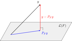
Least squares is dropping a perpendicular in from onto : is the vector of the model's answers on the training sample, the vector of its errors.
Solving the least squares problem, we drop a perpendicular from the point in the space onto the linear span of the columns of the matrix . Least squares says: find in this subspace the point closest to — that is the projection of onto the linear span, and the matrix that transforms into this projection drops the perpendicular; that is why it is called the projection matrix. is the vector of the model's answers on all the objects of the training sample, approximating the given . The orthogonal projection onto the orthogonal complement is the residual, the vector of the model's errors on all the objects. Clearly the original point would hardly have landed exactly in this subspace: the solution is always some approximation. This is important to understand.
Remark (Orthogonal decompositions). Someone asked: this picture resembles the geometric interpretation of conditional expectation — is it the same property? Rather, this: decomposing a space into two mutually orthogonal subspaces that are orthogonal complements of each other is so general a technique in linear vector spaces that one can run into it in very many places and courses. That is the fundamentality of linear vector spaces, and it is no surprise that you have run into it once again. But I would not look for a direct analogy with conditional expectations now: it is another application of the same technique of orthogonal decomposition.
The solution through the singular value decomposition
How is the pseudoinverse found? In different ways: there are a huge number of numerical methods implemented long ago, thousands of times, and telling how they work is outside our course. But I will drag you through one thing, because it is extremely useful, instructive and will come in handy in many other places.
Theorem (The singular value decomposition). Any matrix can be represented as a singular value decomposition (SVD):
The main properties:
- the matrix is orthogonal, ; the columns are eigenvectors of the matrix ;
- the matrix is orthogonal, ; the columns are eigenvectors of the matrix ;
- the matrix is diagonal, , are the common eigenvalues of the matrices and .
The matrices , of size , and , of size , are very closely related: they have the same eigenvalues. More precisely, we agreed that , both matrices have rank , so the larger matrix has its remaining eigenvalues equal to zero, and the nonzero ones of the two matrices coincide. On the diagonal of are the roots of these common eigenvalues — the singular values of the matrix . You have surely covered the singular value decomposition in courses on linear algebra and numerical methods, so this is a repetition.
Let us substitute this representation into the pseudoinverse. Remember that and are orthogonal: is the identity matrix and goes away at once; when the product is inverted, the cancel, times remains, and they cancel too. Moving to writing in terms of the columns of the matrices and , we get:
Identities: , , .
is a column times a row, a rank-one matrix of the same size as . The pseudoinverse has been represented as a sum of rank-one matrices divided by the singular values. Once the singular value decomposition has been computed, finding the pseudoinverse is no trouble at all. The vector of optimal parameters has been expanded in the basis of eigenvectors of the matrix , and again is in the denominator. The model's answers on the training sample, that is, the orthogonal projection onto the linear span of the columns of , have been expanded in the eigenvectors of the matrix — and note: this is the only one of the four expressions without in the denominator. The norm is again a sum, with in the denominator.
Multicollinearity and the condition number
Let us reason about in the denominator. What is bad about it? Recall the notion of an ill-conditioned matrix — a matrix that has eigenvalues close to zero. If some tends to zero, a large unstable term appears in all the sums but one. You will see the effects of instability when you compute the pseudoinverse, when you compute the parameter vector , and when you compute its norm: it will tend to plus infinity, which is a sign of an unstable solution. But you will see nothing of the kind when you look at how the model approximates the sample: nothing tends to any infinity there, and it will seem to you that the solution is great. Nevertheless it is unstable.
Definition (Multicollinearity). Multicollinearity is a linear dependence among the features. Suppose a linear model has been built; multicollinearity: ; non-uniqueness of the solution: . A special case: , an insufficient sample size.
Manifestations of multicollinearity:
- has zero (or close to zero) eigenvalues ;
- has a large condition number;
- weights that are too large and of different signs;
- the weights cannot be interpreted as the importances of the features;
- instability of the linear model ;
- — overfitting.
A singular value tending to zero says that there is an almost linear dependence between the columns of the matrix, that is, between the features. Were the dependence exact, the eigenvalue would be exactly zero, and we could not invert the matrix at all. Still more insidious is the situation where we can invert it, but the inversion is unstable because of tending to zero in the denominator.
Definition (The condition number). The condition number of an matrix :
When the inverse matrix is multiplied by a vector, , the relative error is amplified by a factor of :
The condition number can be defined in different ways, proving that the definitions are equivalent; in particular, it is the ratio of the maximum eigenvalue to the minimum one. In our case — it is the one we invert — and . Errors in measuring the features and the answers are amplified by a factor of when computing the least squares solution vector . Let the relative measurement error be 1% and the condition number 1000, which may easily happen. Then the relative error of the model's parameter vector may reach 1000% — ten times the quantity itself. Having computed the singular value decomposition, we will see this with our own eyes: sort the eigenvalues in decreasing order, compare the minimum with the maximum, and if the condition number is large, something has to be done.
The problem of multicollinearity is closely tied to overfitting. If the matrix is ill-conditioned, the solution is unstable and poorly interpretable: the norm of the vector starts to tend to infinity, and we see coefficients large in absolute value and of different signs — a sure sign that the features are almost linearly dependent. On training it seems to us that everything is fine, but as soon as we use the model on an independent test sample , the instability shows itself at once.
- Regularization: .
- Feature selection: , .
- Feature transformation: , .
The first strategy is treatment that is, as doctors say, symptomatic: if the norm of the vector runs off to infinity, we do not let it, and from all solutions we choose the solution of minimum norm, the most stable one. The second: since the features are multicollinear and there are features depending on others, let us find independent ones and throw out the rest. The third: move to a smaller number of new features; we will consider it in the last part of the lecture. We solved the least squares problem in the first ten minutes, but considering the properties of the solution we see problems that have to be solved, including by changing the problem statement itself. Today we will look at all three strategies.
Ridge regression
The first strategy: penalize the model for increasing the norm of the weight vector. Among the that give the main functional values close to the minimum there may be too many solutions, and we will choose among them the solution of minimum norm: we add the two criteria with a regularization parameter.
Definition (Ridge regression). A penalty for increasing the norm of the weight vector :
where is a non-negative regularization parameter. The modified least squares solution ( is the «ridge»):
The regularization parameter is sometimes conveniently written as , a factor in front of the regularizer, and sometimes as . We will discuss probabilistic interpretations in the next lecture; for now I will only hint that there will be a Gaussian prior on here, and is in effect its variance. Pulling the variance towards zero is the same as greatly increasing the regularization. Regularization is of course a double-edged sword: too small a does not solve the problem, too large a one drives the solution to zero. Differentiating, we get the addition , and it results in being added to the matrix — a «ridge» along the diagonal. Hence the name: ridge regression.
How will show up in the formulas through the singular value decomposition? Let us repeat everything we did before, with the addition:
The regularization coefficient has been added to in the denominator and has thereby moved the denominator away from zero: if tended to zero, we added to it and solved the problem. And the structure of the solution has stayed exactly the same. Let us check ourselves: with we get the same solution as before. With , , but the solution becomes much more stable. It becomes biased. The properties of bias are discussed in courses of mathematical statistics, where multiple linear regression is covered: the solution of the least squares problem is unbiased but may turn out unstable, and by adding regularization we traded unbiasedness for stability. As a result of this trade we get a more profitable solution, because stability does matter.
Choosing the regularization parameter
What is the advantage of the singular value decomposition? It can be computed once for the matrix , giving the matrices , and — that is a lot of computation, 99% of all the work — and then we can compute , and anything we want very quickly by the formulas, varying at that: the singular value decomposition does not depend on . Too small a — weak regularization, instability; too large — a degenerate, zero solution. A compromise is needed, and we know how to tune such hyperparameters: let us do hold-out.
Definition (Choosing on a control sample). The control sample ;
Computing the functional on the control data times takes operations:
The dependence usually has a characteristic minimum.
At the start the whole sample has to be split into training and control: the training one to build the model, and the control one, not very large, to optimize the regularization coefficient. We compute the criterion on the objects of the control sample, substituting the regularized solution, and get a remarkable formula that gives a very fast way to compute the dependence of the hold-out criterion on . The singular value decomposition is computed once; is multiplied once, also once. Now, having this matrix and this vector, one can easily and quickly compute the criterion for any : take on a grid, plot , see the characteristic minimum, choose the optimal . That is the charm of the singular value decomposition: having computed it once, we learn a great deal about the properties of the solution and get the ability to optimize the regularization coefficient.
Regularization reduces the «effective dimension»
Terminology: such regularization is also called shrinkage or weight decay:
People also say that a reduction of the effective dimension takes place in it. But we did not seem to reduce any dimension: we used features and keep using them. Why do people say this? There is an amusing fact: when a projection matrix projects a vector onto a subspace of smaller dimension, the trace of the projection matrix is the dimension of this subspace. The proof is trivial: under the trace sign matrices can be permuted, , after which cancels with its inverse, and the trace of the identity matrix remains:
Let us do the same with regularization. We get a similar construction with the addition ; it is not a projection matrix in the strict sense, it does not do an orthogonal projection, but it still looks for a vector in the space of linear combinations of the columns of :
With we would again get , while leads to a decrease in the trace. The trace here is not a dimension — it is not even an integer — but it is a kind of analogue of one, which is why people say the effective dimension decreases. Regularization squeezes the solution into a neighbourhood of zero: the norm of the weight vector shrinks, and a kind of analogue of the dimension decreases too. An amusing fact, needed just to understand the geometry of what is happening.
LASSO and non-smooth regularizers
So far we added the sum of squares to the functional. Can we add a sum of absolute values? We can. We have already discussed such a regularizer when we talked about its probabilistic interpretation, and today we have a regression problem.
This is LASSO, Least Absolute Shrinkage and Selection Operator. The name, of course, is fitted to the acronym, but the metaphor is rich and memorable: it is as if we throw a noose over the coefficient vector, and it is forced to get rid of excess degrees of freedom. Why can minimization with such a regularizer lead to some becoming zero? And a zero in a linear model means that the feature is always multiplied by zero and is no longer used — this is feature selection, that very second strategy.
For the unconstrained minimization problem with an regularizer there are methods of its own, but there is also a technique that reduces it to a smooth one. The first step: this statement is equivalent to a statement with an inequality constraint, where the regularization parameter is replaced by an upper bound :
There is a monotonic dependence between and ; which exactly we do not discuss now, but the main thing is that for a given one can compute a for which the problems are equivalent. I will not prove it; the idea is this: write out the Karush–Kuhn–Tucker conditions for the problem with an inequality constraint (recall the last lecture) and make sure the resulting system is equivalent to the system of conditions for the original problem.
The second step: make the change of variables , where both terms are non-negative and one of them is always zero. If , then and ; if , the other way round. Then the absolute value is expressed through the sum, , and we get a smooth problem:
It can be solved with the same Karush–Kuhn–Tucker conditions, and complementary slackness conditions appear: the inequality constraints hold as equalities, they rest against their bounds. If we increase the regularization coefficient , more and more constraints will rest against zero: it is profitable for us to decrease the sum of absolute values, that is, the sum . More and more often it will turn out for some that both and , but then too: the feature drops out of the model simply because its coefficient becomes zero. This is hard zeroing. Nothing of the kind happens in ridge regression: there the coefficients may tend to zero but never become exactly zero. This is the radical difference between and regularization.


The typical dependence of the weights on the regularization parameter (schematic). In ridge regression all the weights decrease smoothly but do not reach zero; in LASSO they become zero one after another.
Let us look at some regression problem: the coefficients as functions of the regularization coefficient, which here is also often called the selectivity parameter: the larger , the stronger the regularization and the fewer features remain; selectivity strengthens the selection. In ridge regression, as the coefficient increases, all the begin to decrease, tend to zero, but never reach it. In LASSO, as increases, the coefficients of the features become zero one after another — that is how the noose works. In the end it has strangled all the coefficients; the model is over-regularized and has degenerated into a constant. At the start, with weak regularization, all the coefficients are nonzero, and the model is richest; in between are the intermediate variants. Like the regularization coefficient in ridge regression, in LASSO can be chosen, and there are methods for this — that is a separate story I am not telling. Some compromise variant will throw out part of the features; that is the main property of LASSO regularization. It is also called Tibshirani's lasso, after the author's surname. A good book where this can be found is The Elements of Statistical Learning, in effect the classic university textbook on machine learning, republished many times.
A geometric interpretation of feature selection
One more view of why regularization selects features. Take the equivalent statement: the least squares criterion is minimized under an inequality constraint on the or norm of the weight vector, which cannot exceed the threshold .
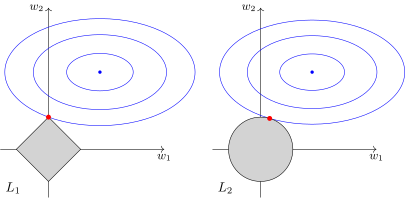
The blue ellipses are the level lines of ; the point at their centre is the unstable global minimum outside the admissible region. The grey region is (left) and (right). The red point is the solution, where a level line touches the admissible region: on the diamond, at a vertex, where ; on the disc, with the same level lines, near the axis but with .
The grey region is the region of admissible solutions. The ellipses are the level lines of , and the global minimum of is outside the allowed zone: it is that very unstable solution. So we look for the minimum only over the grey region the regularizer allows us. For it is a diamond, and look how interesting: wherever the quadratic form is located, the touching most often happens at a vertex of the diamond, on one of the axes — and there one of the coordinates becomes zero. For the region is a disc, and however we move the quadratic form around the space, only on a set of measure zero will we hit points where zeroing happens. In fact we will never hit them, among other things because of computational errors. Here is a vivid picture of why the norm leads to coefficients becoming zero, to feature selection.
One can generalize and take not necessarily or but other norms , and look at what their equidistant surfaces look like — the points at a given distance from the origin. is simply the number of features used: we use one feature, either this one or that one. has a concave shape, and it will have greater selectivity: as the quadratic form is moved, touching at the vertices will happen more often. With and with , the uniform norm, there will be no feature selection.
Non-smooth regularizers for selecting and grouping features
If the model is linear, the , and even norms play the role of shrinkage. In general a regularizer is some function , which one can try taking in different ways.
Definition (Non-smooth regularizers). The general form ( is the selectivity parameter):
- LASSO (): ;
- Elastic Net: ;
- Support Feature Machine (SFM):
Elastic Net is a very useful thing, the sum of the and norms. Why is singled out separately here? Increasing it leads to feature selection, but among the selected features there may still be linearly dependent ones: we allow such multicollinearity but suppress it with regularization. The regularization coefficient and the selectivity parameter are slightly different parameters here, and the features are suppressed less aggressively. It can be done differently too: the methods I told you about at the end of the last lecture, the Support Feature Machine and the Relevance Feature Machine, define the regularization function differently. The main thing is that the regularizer must be non-smooth: if it has this sharp nose, however we construct it, there will be feature selection. Non-smoothness of the regularizer gives feature selection.
Principal component analysis
Let us devote the last third of the lecture to another problem with least squares, now — transforming the feature space. This is the third strategy for fighting multicollinearity. The first is to shrink the coefficient vector; the second, to zero some coefficients, throw out features; the third, to move to a smaller number of new features while preserving the information about the objects. This is a separate problem statement, and the answers are not needed at all in it: we work only with the «objects–features» matrix, and it does not matter to us whether we are going to solve a classification problem, a regression problem, or need a new feature representation of the objects for something else.
Definition (Principal component analysis (PCA)). Given: a sample of objects ; are the numerical features of the objects.
Find: , new numerical features, , and a linear reconstruction of the old features from the new ones:
Criterion — the accuracy of reconstructing on the training sample:
The feature transformation problem is an unsupervised learning problem: there are no answers here.
We want to find a space of smaller dimension that would represent the original objects more efficiently, with an explicit transition from the original space to the new one: the new features must be expressed explicitly through the x's. We want the reverse transition to be possible too: so that the old features can be reconstructed from the new ones, losing as little accuracy as possible. How to reconstruct — a model has to be set. If the model is linear, we get principal component analysis; with a nonlinear model we get other methods, which also exist, but we will not talk about them today. A linear combination of the new features with coefficients , unknown for now, should give, of course, not exactly the original features but their estimates , and we require the estimates to be as accurate as possible on all the objects of the training sample — least squares, a sum over all the features and all the objects. The criterion must be minimized simultaneously over the new features and over the coefficients , that is, we must find both the new features and the way to reconstruct the old ones from them.
Definition (The low-rank matrix decomposition problem). The «objects–features» matrices, old and new:
The matrix of the linear transformation of the new features into the old ones:
The criterion in matrix form — we look for and simultaneously:
The rows of multiplied by the columns of — linear combinations of the new features — must give the old features: must be as close to as possible. Both matrices are unknown. We approximate by a product of two matrices of a smaller intermediate dimension , so the rank of is at most . Let us agree that we solve the problem to obtain linearly independent new features — then this is a matrix of rank . If were also of rank , the representation would be exact; but if all the matrices have full rank, it is a matter of approximating by a product of two matrices of lower rank, that is, of a low-rank matrix decomposition.
Theorem (The main theorem of principal component analysis). If , then the minimum of is reached when the columns of are the eigenvectors of the matrix corresponding to the largest eigenvalues , and the matrix . Moreover:
- the matrix is orthonormal: ;
- the matrix is orthogonal: ;
- ; ;
- .
Identity: .
Look carefully at this set of conditions: you have already seen it somewhere today. The new features are also expressed linearly through the old ones, by the ready formula . If we write out column by column, we get — the condition that is an eigenvector of the matrix ; the matrix notation says that the columns of are orthonormal eigenvectors of . Similarly the columns of are orthogonal eigenvectors of the matrix . Look how interesting: the columns of are the new features, and they are orthogonal as vectors of values on the objects of the training sample. That is why the transformation is also called orthogonalization.
And the last, important property is the accuracy of reconstruction. The squared norm of a matrix equals the sum of its eigenvalues, and the squared norm of the difference, the accuracy of the matrix decomposition, turns out to be the sum of the smallest eigenvalues. Now it is clear why the method is called principal component analysis: for the residual to be minimal and the accuracy of reconstruction maximal, we must take the largest eigenvalues, because the decomposition error equals the sum of the remaining ones. The largest eigenvalues and the eigenvectors corresponding to them are called the principal components: they contain the maximum of information about the original matrix .
The link with the singular value decomposition
Up to notation, I think you have already seen the link with the singular value decomposition.
Proposition. Any matrix can be represented as an SVD: , , , . If we take , then:
- ;
- the representation is exact and coincides with the SVD if we set , : ;
- the linear transformation works both ways: ; .
— the new features are uncorrelated; is the decorrelating Karhunen–Loève transformation.
If the dimension is not reduced, the sum of the remaining consists of zero terms, and the representation is exact. It coincides with the singular value decomposition if is represented as the product of an orthonormal matrix and a diagonal one with the roots of the eigenvalues on the diagonal. The transformation works both ways: on the right of gives , on the right of gives , because here is . And since the new features are uncorrelated, this is also the Karhunen–Loève transformation. Principal component analysis was probably reinvented dozens of times over the decades: it appeared in very different problems, in different notation, people derived everything anew and ended up arriving at it.
The effective dimension of a sample
When does principal component analysis bring benefit, and when is it useless? It brings benefit when there are linearly dependent features among the features. That means the sample is in fact distributed not over the whole space but lies in a subspace of smaller dimension. Principal component analysis moves explicitly into this subspace and finds a new basis in it — new features, the matrix — an orthogonal one even, which is very convenient. The original problem can now be reformulated in these features.
Definition (The effective dimension of a sample). Order the eigenvalues of in decreasing order: . The effective dimension of the sample is the smallest integer for which
The «steep slope» criterion: find for which .
The «steep slope» criterion (slide): the effective dimension is where .
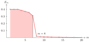
The «steep slope» criterion: the relative reconstruction error drops sharply from to and hardly changes after that. So the sample lies in a subspace of dimension . The values are read off the slide by eye.
How can we tell whether the sample lies in a subspace of smaller dimension? With the same spectrum. The relative error — the squared norm of the difference divided by the squared norm of , that is, the sum of the smallest eigenvalues divided by the sum of all — is a very convenient quantity from zero to one, and it can be plotted. If in one place a sharp drop has occurred, followed by a tail where the relative errors are already small and can be neglected, then the point of the drop is the dimension at which the error dropped sharply, and a further increase in the dimension of the subspace will not lead to a significant improvement in accuracy. So is the dimension of the space in which our sample is actually located.
Is it always so? Of course not. In many problems the plot is a monotonically decreasing function, decreasing to the end and never reaching values close to zero. Then the sample lives in a space of full dimension, and applying principal component analysis to it is useless and incorrect. We found the singular value decomposition, plotted the spectrum, and look at it with our eyes: is there a steep slope? If there is, then there are reasons why the sample ended up in a space of smaller dimension. For example, we constructed the features in such a way that some implicitly depend almost linearly on the rest, and we did not catch this dependence — we lacked the imagination to invent independent features. This happens fairly often, so it really does make sense to look at the dimension of the subspace the sample actually lives in.
Principal component analysis in linear regression
We have considered two problems: supervised learning, multiple linear regression, and unsupervised learning, principal component analysis. We solved both by least squares, understood their properties, and both are deeply tied to the singular value decomposition. Let us put a bold full stop here, take a deep breath — and now apply principal component analysis to solving the problem of multiple linear regression.
Definition (Solving the least squares problem in the new features). Replace with its approximation , assuming :
The link between the new and old coefficient vectors: ; .
The solution of the least squares problem with respect to :
The only difference from the former is terms instead of .
is the new parameter vector, now over the new features, and is our new model. We found and , threw the original away, and solve the least squares problem with the new feature matrix ; between the new and old coefficient vectors there is a linear link following from the properties of principal component analysis. And principal component analysis is expressed through the same singular value decomposition, only in it one has to take the largest eigenvalues and throw away the rest. The form of the solution is the same. Recall what ridge regression was for: to move the away from zero, and we added to them. Now we move them away from zero differently: we simply throw the eigenvalues close to zero out of all the expressions as terms. This is equivalent to principal component analysis. An interesting link: both regularization and principal component analysis in the solution of the least squares problem are the same decompositions, in which we move the spectrum away from zero by different techniques.
The spectral method of least squares
This leads us to a mega-generalization of least squares. Having expressed least squares through the singular value decomposition, we understood how regularization is expressed through the SVD, and then that principal component analysis is expressed through the SVD. The structure of the solutions is absolutely identical; the only difference is how we move the small away from zero. A generalization comes to mind at once.
Definition (The spectral method of least squares).
- Build the SVD decomposition, order .
- Move the smallest eigenvalues away from zero: . Special cases:
- — ridge regression;
- — principal component analysis;
- — something in between.
- Apply the SVD formulas to modify the least squares solution:
We keep all the eigenvectors, we keep the structure of the solution. Ridge regression is the special case where is added to all the eigenvalues. But if an eigenvalue was large, why add to it? We need not: the main thing is that the small ones are moved away from zero. Principal component analysis is as if we added infinity to the small , that is, zeroed the corresponding terms in the sums where is in the denominator. Something in between can also be done, in different ways. There are many variants of how to set the additions ; they can be invented and then the question posed: which of these spectral solutions suits us better for some reason? Such is the mega-generalization, not at all obvious: it would have been hard to guess it from the start. We arrived at it by comparing ridge regression with substituting principal component analysis into the solution of the least squares problem and noticing that the structure of these solutions is the same.
Low-rank decompositions: what comes next
And a spoiler of what lies ahead: in the second semester there will be a lecture on recommender systems, and a few more occasions to talk about low-rank decompositions. Principal component analysis is not the only statement.
Definition (Sparse low-rank matrix decomposition). Given: a matrix known only in the cells .
Find: the matrices and .
Criterion:
Very often the matrix is given not in full but only on some subset of cells: missing values — for some objects not all features could be measured. The classical singular value decomposition assumes the matrix is fully known; there can be no gaps in it, and it is not even clear how to handle them. But there are more modern methods that solve such a problem explicitly: the sum of squares is still minimized, but only over the cells for which there are observations. It can be solved, for example, by the stochastic gradient method. This is of course no longer the SVD, and there will be no orthogonality properties for and . The matrix is sparse, known only on a subset of values, and it is represented by a product of two dense matrices of lower rank, where there are no gaps any more. There are other variants too: a loss function that is not quadratic, additional non-negativity conditions. This is just a spoiler, so that you feel what other problem statements there are — things by no means end with principal component analysis.
Summary
Today we realised a very interesting role of the singular value decomposition. With it one can solve the problem of multiple linear regression; one can insert regularization, ridge regression, into it — also through the singular value decomposition; one can do principal component analysis — also through the singular value decomposition; and one can combine principal component analysis with the solution of the multiple linear regression problem and also get a solution through the singular value decomposition. Such an interesting and fairly general thing.
Remark (How to interpret the principal components). After the lecture someone asked: is there a technique for explaining what new features we have obtained — roughly speaking, to a marketer? It does not always work. What is known about the new features is that there are fewer of them than of the old ones; that they are orthogonal to each other; that they are linear combinations of the original features; and that they are optimal features that make the reconstruction of the original data as accurate as possible. Nothing more is known. Orthogonality is very convenient mathematically, especially in linear problems where is needed and is a diagonal matrix, what luck. But this ease is purely mathematical. You say: the new features are orthogonal — and the marketer looks at you with square eyes: what does orthogonal mean, why do I need it, what properties do the new features have? There may or may not be meaningful substance in this. What these linear combinations represent in terms of the meaning of the original features is not always clear. So the question in general hangs in the air, and it is the question of whether the method should be applied at all.
A partial answer is this. If the effective dimension turns out to be very small, say two or three, that is simply wonderful: you have managed to represent the whole sample in a two-dimensional space. Two new features — who knows what clever weighted sums of the original ones — but all the data fitted into them very well. Then you build a two-dimensional plot in the axes of these two features, draw the sample on it, and sometimes you understand what these axes are. Long ago we took the results of the elections to the State Duma, of 1995 I believe — at that time there were more than forty political parties. The matrix: how many people in each region voted for each party; the regions are objects, the parties are features. Principal component analysis showed that the whole sample fitted very well onto a two-dimensional plane. Along one axis lay the political spectrum from communists to libertarians, along the orthogonal one from nationalists to internationalists: at that moment, on those data, these turned out to be the two main axes of the political spectrum. An attempt to single out a third axis led to nothing sensible: the third eigenvalue was already much smaller than the first two, and the spread of the data was mainly described by two axes. This is an example where principal component analysis turned out quite interpretable, but that is far from what happens in all applied problems.
And if the sample is large but fits into a space of smaller dimension, there is always something interesting behind this fact. Even if the first component turns out to be a strange combination of the original features, it makes sense to try, together with experts in the subject area, to find a sensible interpretation: such a fact is nontrivial, and there may be a discovery behind it from the point of view of the subject area.
No comments yet
Be the first to share your thoughts.