August 30, 2026 · Lecture · LibreTimes
Machine Learning 1. Lecture 4. Metric Methods of Classification and Regression
Contents
- What this lecture is about
- The continuity and compactness hypotheses
- How to measure distances between objects
- The generalized metric classifier
- The k nearest neighbours method
- Weighted neighbours and the Parzen window method
- The method of potential functions
- Potential functions as a linear classifier
- Complete cross-validation and the compactness profile
- The proof
- Properties of the compactness profile and the CCV estimate
- Prototype selection
- Nonparametric regression: kernel smoothing
- Choosing the kernel and the window width
- The problem of outliers
- Summary
- Seminar
What this lecture is about
Today, metric methods of supervised learning. They are probably the simplest methods in machine learning: what could be simpler than the nearest neighbour method? On the other hand, year after year I kept adding things to this lecture — it seemed very simple to me, so I added one interesting thing, then another — and as a result today's material is dense. Hold on, but you will learn a lot of interesting things.
The continuity and compactness hypotheses
Let us start with a very simple paradigm. In regression, when we recover one numerical quantity as a function of other numerical quantities, it seems that in nature we most often meet continuous functions. So the assumption that the dependence being recovered is continuous is, if not the most frequent, then the most obvious of everything that can occur.
Definition (The continuity and compactness hypotheses). are the objects, the answers, the training sample.
The continuity hypothesis (for regression): close objects have close answers.
The «compactness» hypothesis (for classification): close objects, as a rule, lie in the same class.
There are samples where clearly depends continuously on , and there are samples that are who knows what, some chaos, and it is not obvious whether there is any functional dependence at all. For classification problems the notion changes slightly, and since the sixties, including in the Russian literature, the term compactness hypothesis has been established. Compactness here is understood in the everyday sense, not at all in the sense of the definitions from courses in mathematical and functional analysis: what is meant is that classes are compact clumps of points. If the classes are mixed with each other chaotically, then it is probably some wrong problem: either the metric was introduced wrongly, or there are many errors in the data — in short, something is wrong with it.
The classic example is Fisher's irises: three classes of 50 specimens each, four features plotted against each other pairwise. One sees very well what we mean when we say that classes are compact clumps of points: here is one clump, here are two others, a little less separated from each other. If the clumps are well separated from each other, the problem is easy, and it probably does not even matter much which models we use to separate the classes — everything will work out well.
How to measure distances between objects
Let us get used to the terms. Of a distance function between two objects, as a rule, only non-negativity is required. A metric is a little more: it has an important property, the triangle inequality. When we say «metric methods of classification and regression», we mean that a distance function has been introduced, which is as a rule a metric. None of the methods explicitly requires the triangle inequality, and we will not talk about it further. But if it does not hold, it is intuitively clear that the distance function is somehow not quite right and may behave wrongly. So we mostly use metrics.
Definition (The Minkowski metric). The Euclidean metric and the generalized Minkowski metric:
where is the feature vector of the object , is the feature vector of the object ; are the weights of the features (possibly learnable).
The first thing that comes to mind is the Euclidean metric in : squared differences, a square root; we have all long been used to it. In the generalized metric, parameters are introduced. The feature weights play two roles. The first is normalization, bringing features to a common scale: if one feature is measured in fractions of a unit and another in billions, then when they are added directly the second will simply drown out the first, and the first will not be visible against it. The second is setting the degree of importance, the informativeness, of the features. Another generalization is the exponent : it need not be two. The geometry of the metric space depends on — what the level lines look like, the sets of points equidistant from a given one.
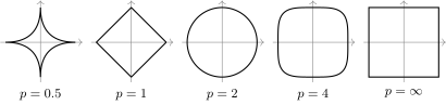
The level lines (equidistant surfaces) of the Minkowski metric on the plane for different : for a circle, for a diamond, for a square, for a concave «star».
This is not the only way to introduce distances; we will not deal with such things further in the course, but so that you know what exists in the world. There are lots of problems on symbol strings, in particular many problems of bioinformatics, where there is a natural definition of the distance between strings. The simplest is the edit distance (the Levenshtein distance): how many insertions, substitutions and deletions have to be made to turn one string into another.
Something similar is done with signals. For example, in recognizing signatures or handwriting written with an electronic pen, the object is described by several curves: the coordinates of the pen, the direction of its motion, the azimuth; one could also introduce speed, tilt angle, pressure. How do we compare two handwritten letters? Take their signals and imagine that little springs are stretched between nearby points of the signals. To bring one signal to the other, some springs have to be compressed and some stretched; the energy of compression and stretching is the distance between the signals. Such methods are called alignment: one can align symbol sequences, and one can align signals. Images are compared in the same way, faces for example: we stretch a mesh over a face, each edge of which is a little spring, and compute the energy of compression and stretching needed to make one face from another. For similar faces this energy is small.
A signal or a symbol sequence can be of arbitrary length, and generating from it a vector of a fixed number of features (feature generation) is rather difficult. But measuring the distance between such objects directly may be much simpler. So metric methods can in general be feature-free: we can compute distances between objects but do not know any features.
Remark (How the edit distance is found). Someone asked: the edit distance seems ambiguous — there are many ways to make the insertions — so is there a search for a shortest path on a big graph of solutions behind it? In principle that is so. If the texts are very dissimilar, there will be many variants, and the variant with the minimum energy is chosen — with the minimum number of substitutions, insertions and deletions. But text comparison programs and a huge number of bioinformatics algorithms exploit the fact that most often we compare strings that are already similar to each other and differ by local changes: different versions of the same program code, similar proteins, amino acid or nucleotide sequences. The prior similarity of the strings simplifies the problem greatly, sometimes to the point where the edit distance is found unambiguously by a fairly simple heuristic algorithm. The algorithms themselves are fairly complex and not material for our course: the examples here are to justify that sometimes measuring the distance between objects is simpler than inventing their features.
The generalized metric classifier
Let us start with classification methods under the condition that we can measure the distance from any object to any object of the training sample . Let us agree on notation.
Definition (The generalized metric classifier). For an arbitrary , rank the objects by increasing distance to :
is the th neighbour of the object among ; is the answer on the th neighbour of the object .
A metric classification algorithm assigns the object to the class to which its nearest neighbours belong:
where is the weight, the degree of closeness of its th neighbour to the object , non-negative and non-increasing in ; is an estimate of the closeness of the object to the class .
I begin straight away with the generalization; the other methods will be special cases. This is a heuristic, and it somewhat diverges from what I have been instilling in you since the first lecture: that we always write out an optimization criterion and find the model parameters by optimizing it. Not so here. This is the rarest case in machine learning where we build an algorithm without an optimization problem, which is why I say that metric algorithms are the simplest: no explicit optimization even takes place here. One could, of course, pose the inverse problem: construct the optimization functional that we implicitly optimize by writing out such an algorithm. That is not homework, but whoever is interested — try it as an exercise.
What does the algorithm consist of? We assign the object to the class whose objects are closest. We rank all the objects relative to by increasing distance and see which class has more objects among its neighbours. The degrees of closeness of the neighbours are summed separately for each class — the square bracket says we sum only over the objects of class — and we get . Everything depends on how the function is defined, and it can be defined in different ways; substituting different definitions into this formula, we will get different heuristic metric classification methods.
The nearest neighbours method
The simplest special case is the nearest neighbour method: the weight is one only for the first neighbour and zero for the others. What is bad about the first nearest neighbour? That it may by chance be in the wrong class. We should look at a neighbourhood of nearest neighbours and vote on which class has more. That is the nearest neighbours method ( nearest neighbours, NN) — voting over the nearest neighbours:
The method is very easy to implement. There is even a name for it — lazy learning: training comes down to memorizing the sample. In essence the method has one parameter, , and it can be optimized. For this there is the criterion we talked about in the first lecture — leave-one-out:
We take as training objects the whole sample except one object , exclude it from all neighbourhoods and see whether it was classified correctly. By the minimum number of errors we determine the optimal . A small is bad because noisy data affects the result; a large is bad because we look at too large a neighbourhood and oversmooth. Somewhere in the middle an optimal can always be found.
LOO against the number of neighbours on the Iris problem (slide): in blue, the biased number of errors, when an object counts as its own neighbour; in red, the unbiased one.
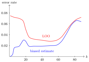
Fisher's irises: the error rate of the nearest neighbours method against . In red, the unbiased LOO estimate; in blue, the biased one, when an object counts as its own neighbour. The curves are smoothed and read off the slide by eye.
If in the implementation you make a mistake and forget to exclude the object from its own neighbourhood, you get a biased estimate. It will seem to us that the optimum is , and it is clear why: on its own an object is always classified without error. What is unexpected here is that the bias persists for a very long time: even at large a systematic gap remains between the blue and red curves. Leave-one-out is a cool thing, but if you forget to exclude the object from the neighbourhood, everything stops working, and the optimal number of neighbours cannot be determined from the biased estimate. The object must be a control one.
The red curve also shows that the optimum is fairly wide: the data is noisy, but it does not matter how precisely the optimum is determined. Choosing parameters by leave-one-out occurs fairly often in machine learning, which is why I am talking about this plot for so long: remember that for many parameters LOO gives a characteristic optimum. It is good when it is wide.
Drawbacks of the nearest neighbours method:
- ambiguous classification when , — if among the nearest neighbours there are equal numbers of objects of different classes;
- the values of the distances are not taken into account. Suppose we take five nearest neighbours, four of them really are the nearest, and the fifth is somewhere out on its own and not a neighbour at all. We ranked the objects by distance, but the distances themselves are not taken into account, and that is probably wrong: the function should depend on them directly.
Weighted neighbours and the Parzen window method
Let us gradually deal with these drawbacks. To prevent ties among the estimates , one can introduce weights that decrease with the neighbour's number: the farther the neighbour, the smaller its weight.
Definition (The weighted nearest neighbours method). , where is a weight that depends only on the neighbour's number; for example,
A linear dependence should not be used. Suppose, for example, there are two classes and four nearest neighbours: the first and fourth in one class, the second and third in the other. The estimates of the classes will be equal. A nonlinear decreasing function is needed, a geometric progression for example, and for two classes the problem is solved. But if there are three classes, ambiguity can still arise. For two classes there is also a simple solution — take an odd number of neighbours — but for three classes it may no longer work.
The next problem: how should the distances to the neighbours be taken into account? It is probably more correct for the weight to depend not on the neighbour's number but explicitly on the distance to it. Let us introduce a decreasing function of the distance — we will call it the kernel — and one more parameter , the bandwidth.
Definition (The Parzen window method). , where is the window width (bandwidth), is the kernel, non-increasing and positive on .
The Parzen window method with a fixed width:
The Parzen window method with a variable width:
The function can even be defined so that it is positive on the interval and zero outside it. Then all the neighbours at distances less than get nonzero weights, and the rest are not taken into account at all. Substituting such a function into the general metric classifier, we see another useful thing: we can get rid of the numbering of objects by neighbourhood altogether. The distances are taken into account explicitly, and the metric algorithm is written as a sum over all the objects of class , where is simply a closeness function.
One unpleasant point. In the nearest neighbours method we guarantee that there will be votes. But a window of width may contain no objects at all. Moreover, at one point of the space the neighbourhood of radius may contain a thousand objects, and at another none. These two ideas can be combined — closeness with a kernel and nearest neighbours — so that a given number of neighbours is guaranteed to fall into any neighbourhood. For this a variable window width is introduced: as we take the distance to the th neighbour. Then the th neighbour will most likely have zero weight, and the first are guaranteed nonzero weights. «Most likely» — assuming that all the distances are different.
By LOO one can optimize the window width , if it is fixed, and the number of neighbours , and also choose the kernel . The plots have a characteristic minimum both in and in .
Example (The effect of the window width). A two-dimensional model sample, , : one class is generated from a Gaussian distribution with a large variance, the other with a small one, so that the classes overlap and there are points that cannot be clearly assigned to a class. The kernel is Gaussian, ; for two classes
With a very small window width, (the side of the square shown is 6), with a Gaussian kernel essentially only the first neighbour gets a large weight; the weights of further neighbours tend to zero. This is very similar to the one nearest neighbour method, and the boundary between the classes comes out very jagged. Each straight segment of it is determined by two points, one from each class — it is the perpendicular to the segment between them. The surface looks very much piecewise linear, but complicated. With the separating surface becomes smoother, though traces of the segments determined by pairs of nearest points are still visible. With it is already a practically round region of the green class. As grows further, the surface tends to one of very low curvature, a linear one.
The method of potential functions
Let us look at the Parzen window method and realise the following. We stood at the point , the object to be classified, looked at its neighbourhood — nearest neighbours or of radius — and saw objects of which classes fall into it. One can look at the problem dually: stand at each object of the training sample and say that it spreads the potential of its class around itself over a neighbourhood of some radius. With each point of the training sample we associate two parameters: the radius of the potential and its amplitude . The method now has parameters.
Definition (The method of potential functions). , or, in a simpler notation where the objects need not be ranked,
where are the weights of the objects, .
M. A. Aizerman, E. M. Braverman, L. I. Rozonoer. The Method of Potential Functions in the Theory of Machine Learning. 1970 (in Russian).
The analogy with electrostatics is very vivid: is the size of the «charge» at the point , the «range» of the potential centred at , and the sign of the charge. In physics there are only two classes, charges or , and from physics one can even take a formula for the kernel, or . But this is of course pure heuristics: in our case the kernel is an arbitrary decreasing function, and there is no reason to take it from electrostatics in particular. In classification problems there are no restrictions either on or on the number of classes. And if there are many classes, the analogy is more with a smell: each point spreads the smell of its class, and we stand at the point , sniff and try to understand which class we are closer to.
Potential functions as a linear classifier
Another important insight: the method of potential functions can be written as a linear classifier. It would seem that the two methods were proposed from completely different heuristic principles. A linear classifier is a separating hyperplane; potential functions are the compactness hypothesis, a metric, converting distance into closeness. Yet the result turns out very similar. In the case of two classes, :
Here is an estimate of how close the objects of class are to , minus the same estimate for class . We took account of the minus in front of the sum over the objects of class by multiplying by . Compare with the linear classification model:
- are new features of the object , the closeness (similarity) of the object and the training object ;
- are the weights of the linear classifier;
- : the number of features equals the number of training objects.
An interesting and unexpected turn. We always talked about the «objects–features» matrix, objects and features, while in metric methods there were initially no features, only distances between objects. It turns out that the distance from the object being classified to a training object, as a function of , can be treated as a feature, and if we make closeness out of distance with a kernel — also a feature. The features are moreover parametrized: the radius sits in them, which would have to be determined somehow. But if we have estimated or roughly determined it somehow — for example, as the distance to the tenth neighbour, or such that the neighbourhood contains mainly objects of one class — and fixed it, then the method of potential functions becomes a linear classifier: the features are the closenesses to the objects of the training sample, the weights are the amplitudes of the potentials . Now it is clear how to train such a method: as a linear classifier over these features, having formed the «objects–features» matrix explicitly.
An idea arises at once: perhaps there is no need to compute closenesses to all the objects of the training sample, and it is enough to take a subset of prototypes and compute distances only to them? The sample may contain a million objects, and we will take, say, a hundred typical representatives in each class and cut the volume of stored data by a factor of 10,000. Why store all the objects if one can keep only those sufficient for reliable classification? We will now work this idea out and along the way get acquainted with an interesting theory.
Complete cross-validation and the compactness profile
This is an element of the combinatorial theory of generalization ability, which makes it possible to obtain criteria of the leave-one-out type, and even complete cross-validation, by an elegant, efficiently computable formula. There will even be one proved theorem here. For my course this is a little unusual; further on I will not refer much to generalization theory. But this insertion is in place here: it gives a logical transition to prototype selection methods — how to select from the training sample a small number of objects sufficient to classify all the others. For this we will need efficient formulas for computing cross-validation.
Definition (Complete cross-validation). Complete cross-validation (CCV):
is the error rate of the algorithm on the control sample , averaged over all partitions of the sample into a training subsample and a control one .
We take the original sample and split it in all possible ways into a training part and a control part . Note: here is new notation, the length of the control sample, not the number of nearest neighbours. is the number of all ways of making such a split. On each split we compute the share of the objects of the control sample on which the algorithm trained on the training sample errs, and we average these error shares. Cross-validation in general is splitting the sample into train and test; when the splits are all possible ones, it is complete cross-validation. Computationally the thing is very inefficient, especially for large : there may be astronomically many splits, and we will not compute this sum explicitly. For we get our old acquaintance: , there are only splits, and the computation can be done directly.
The problem: obtain an efficiently computable formula for the complete cross-validation of the one nearest neighbour method and answer the question of whether the 1NN method can be improved by minimizing CCV. You will say: what can be changed in the one nearest neighbour method? To run ahead: the set of prototypes. One can throw out of the training sample the objects not needed for classification and keep the part that optimizes generalization ability in the sense of complete cross-validation. This is no longer quite lazy learning: training will consist in selecting the most important objects. But first we need a formula for CCV computed more efficiently than by full summation over partitions. Can we get away from summing over partitions? We can, and first we need a definition that formalizes that very compactness hypothesis.
Definition (The compactness profile). The compactness profile of the sample is the share of objects whose th neighbour lies in another class:
where is the th neighbour of the object in and is the answer on the th neighbour of the object .
In meaning, this is exactly the formalization of the compactness hypothesis: if the classes are compact clumps of points, then for each object most of its nearest neighbours lie in the same class, and is close to zero for small .
Theorem (The exact expression of CCV for the 1NN method).
K. V. Vorontsov. A combinatorial approach to estimating the quality of learning algorithms. 2004 (in Russian).
I managed to obtain this result when I was working on generalization theory for my doctoral dissertation. It is interesting not only because it formalizes the notion of compactness explicitly, as the compactness profile of the sample, but also because it gives a method of prototype selection.
Compactness profiles for a series of model problems (slide): top row, the samples; middle, the compactness profile ; bottom, against the control length .
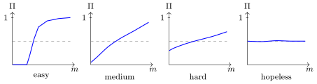
The compactness profiles for a series of model problems on 200 objects, from classes far apart to classes mixed chaotically. For the nearest neighbour method the initial part of the profile matters. The curves are smoothed and read off the slide by eye.
Example (The compactness profiles of model problems). In the first problem the classes are far from each other — an ideally easy problem for nearest neighbour methods. For all objects the first 50 nearest neighbours lie in their own class, and there will be no errors either with one nearest neighbour or with 20. Let us make the problem harder: the classes are moved closer, and the initial part of the profile — and we are interested precisely in the profile at small — has risen: the classes have begun to penetrate each other, and there will be more errors. When there is no hope of solving the problem with acceptable quality by nearest neighbour type methods, the compactness profile is somewhere around : that is random guessing.
Another row of plots on this slide shows how complete cross-validation depends on the length of the control sample , and the result is very good for us: it does not depend on it very strongly. For small the spread is slightly larger, but the control length can quite well be taken small. This is a very optimistic experimental result: there is no particular reason to put more than one object into the control sample, and LOO can be used. This was not obvious from the start.
The proof
The proof is not difficult, rather beautiful, and shows how theorems about generalization ability — about how a method trained on some data will work on new data — can be proved by combinatorial methods at all. Under a finite sample such a prediction can be made.
Proof. The main idea is to sum over the partitions analytically. Let us write CCV summing over all the objects of the combined sample, but counting only the objects of the control part:
Why can an error occur on the th object? The object is classified by its nearest neighbour in the training sample — say, by its th neighbour in the whole sample. How could it happen that precisely the th neighbour ended up in the training sample and became the nearest? All the previous neighbours must have ended up in the control sample, together with itself. For a given partition we do not know which of the neighbours turned out to be that th one, so we formally introduce an additional sum over :
Now the favourite combinatorial trick — swap the summation signs:
The inner sum is the number of partitions in which one particular object, the th neighbour of the object , went to training and more particular objects went to control. We know this number: the remaining objects are distributed so that of them go to training, that is, it equals . The rest is easy: what remains together with the summation over is the compactness profile, and the combinatorial factors combine into one:
The reasoning is fairly simple, but it relies essentially on this being the method of one, the first, nearest neighbour. A similar theorem can be proved for nearest neighbours: technically a little more complicated, but in essence the same combinatorics. However, combinatorial bounds on generalization ability can be obtained for few machine learning methods: it is rather the exception.
Properties of the compactness profile and the CCV estimate
Let us denote the combinatorial factor
- faster than a geometric progression:
So in the compactness profile only at small matter for the estimate.
- A formalization of the compactness hypothesis: the more often close objects lie in the same class, the smaller CCV.
- For small :
At , , , begin to be counted, but with very small weights, and the main contribution comes from , that is, LOO.
- CCV depends weakly on the control length .
Along the way we have justified — true, only for metric nearest neighbour methods — that leave-one-out can be used: this estimate is unbiased and depends little on the control length, which is also good news.
Prototype selection
What did we obtain all this for? To learn, in the nearest neighbour method, to get rid of the training sample: to throw out most of its objects so that what remains are prototypes, representatives of their classes, by which all the other objects can be classified successfully. In English this is prototype learning, and there are hundreds of prototype selection methods: simple and complex, heuristic, optimization-based and many others. One of them is based on bounds through the compactness profile. The definition will have to be modified by introducing a dependence of the profile on the set of prototypes ; this is no more complicated than what we have already done.
Definition (The prototype selection problem). is a 1NN classifier that uses as nearest neighbours only objects from the set . We need to find the optimal subset of prototypes .
The compactness profile relative to :
where is the th neighbour of the object from the set .
Theorem.
where is the contribution of the object to CCV.
It is proved in the same way, only the terms are grouped a little differently in the proof: the contribution of each object to CCV is singled out, if only the subset is used as prototypes — the objects we allow to be nearest neighbours. Two fairly obvious greedy strategies arise.
Definition (Greedy prototype selection by the criterion). The greedy strategy of removing non-prototypes:
- ;
- repeat: find for which ; ; update for all that have among their nearest neighbours;
- while CCV decreases or hardly increases.
The greedy strategy of adding prototypes:
- one object from each class;
- repeat: find for which ; ; update for all that have among their nearest neighbours;
- while CCV decreases.
In the first strategy we look at which object's removal from the set of prototypes changes complete cross-validation least, and successively throw out the most useless objects. In the second we go from the other end: take as a seed, for example, one random object of each class and ask which object it is most profitable to add so that CCV becomes minimal afterwards.
Example (An experiment on synthetic data). Two classes of 500 objects each, generated from two-dimensional Gaussian densities, with 30 noise objects added: white points that ended up inside the black class and black ones inside the white.
Greedy removal of non-prototypes. Three types of objects result. The first to be thrown out are the noise outliers, exactly the 30 we made noisy: throwing them out decreases CCV most. Why? In the neighbourhood of each outlier an error will occur, and it also affects the classification of the objects nearest to it, and errors occur on them too. This shows that the prototype selection strategy works adequately. Then comes a long stage: the bulk, more than 900 objects of both classes, is thrown out. They are useless for classification: they lie deep inside their class, there are no errors on them, they are reliably classified by their neighbours and are not needed to classify their neighbours, because there are many such in the neighbourhood. At the end the prototypes remain, and they have lined up along the boundary between the classes. We did not do this deliberately: it just happened that the algorithm left the objects that can no longer be thrown out — that would strongly affect the value of CCV. Whether it will always be so, or whether it is due to the geometry of this model problem, I have no answer; in problems with a different class geometry the strategy may work differently.
Greedy addition of prototypes. Here an interesting thing happened: the prototypes were added somewhere far from the boundary between the classes. It turned out that in this method it is more profitable to build the boundary from prototypes lying far from it. This too was not built into the method from the start. A curious result: the two strategies work differently. Can they be combined, adding and removing in turn? Probably they can, and there are many such methods too.
CCV against the number of objects removed. I liked the first picture more, where the prototypes stand along the boundary like border guards and separate one class from the other. What was happening with the criterion? When roughly the first 40–50 objects were thrown out, the criterion slowly improved. Then, from roughly the 50th to the 980th, nothing happened to it at all; the changes were minute, invisible to the eye: uninformative points were being thrown out, neither noise nor prototypes, just unneeded for classification. And when roughly the last ten objects were thrown out, CCV shot up: do not touch these objects. About 20 objects are enough to classify this model sample with practically ideal achievable quality. Along the way, on an independent test sample — another 500 + 500 generated objects — it turned out that no overfitting occurs in prototype selection, apparently because complete cross-validation is taken as the criterion.
K. V. Vorontsov, M. N. Ivanov. Prototype selection based on minimizing the complete cross-validation functional. 2009 (in Russian).
The topic of prototype selection arose somewhere in the sixties and was quite popular until the nineties; hundreds of methods have been invented, mostly heuristic. Why so? Prototype selection is a search for an optimal subset in a finite set of points, and that is an NP-hard problem: in general it requires going through an exponential number of subsets. All known algorithms revolve one way or another around how to cut the search time and find a more or less good set of prototypes. And our method, though it rests on a bound on generalization ability — an efficiently computable formula for complete cross-validation — at the moment of optimization solves an NP-hard problem by a heuristic algorithm, successive greedy removal or addition.
So today we generalized the nearest neighbour method and made it nontrivial in two directions. First: we began increasing the number of neighbours, voting, weighting the neighbours, and reached the method of potential functions, which turned out to be a kind of linear classifier with closenesses as features. Here the method remains lazy learning; training comes down to storing the sample. Second: we kept the one nearest neighbour method but threw the bulk of the unneeded objects out of the training sample and kept only the prototypes sufficient for good classification — we posed the optimization problem of keeping the minimum number of prototypes.
Remark (Prototype selection today). Someone asked whether these methods will have to be programmed. No, there are no assignments on this. But it is good to know that machine learning deals not only with solving optimization problems: we can also pose theoretical questions about bounds on generalization ability, and sometimes the bounds lead to criteria that can then be optimized to achieve results, as here with prototype selection. This idea surfaces from time to time even in fairly advanced applications, including with deep neural networks. Recently I saw a paper about an image store for a security system: a company employs thousands of people, their faces have to be recognized, and new employees keep appearing. It is a classification problem with a variable number of classes, and the system must not degrade as it learns more faces. Prototype selection found an application there: one or two photographs are stored for each employee, selected so that quality degrades minimally. I was surprised to find that prototype learning, which seemed to have become obsolete some thirty years ago, still crops up in fairly modern applications.
Telling a combinatorial proof in ten minutes is something of a challenge for me, and understanding it is one for you. There was a sharp turn here, and it is no disaster if something was unclear: it is a deliberate insertion of theoretical material, so that you know that machine learning is not only neural networks and optimizing loss functions but such theories too.
Remark (Merging close objects). After the lecture someone asked: what if, instead of simply removing points, we merge them — put a point of double size at the centre of mass? Yes, there are such methods, learning vector quantization for example, and many have been invented. Compact clumps can be replaced by a single representative — an object of the training sample or some average; it happens both ways, depending on what is simpler to do.
Nonparametric regression: kernel smoothing
Metric regression methods are also called nonparametric — such a random play on words. The simplest of them is kernel smoothing.
Definition (The regression problem and weighted least squares). are the objects (often ), the answers (often , more rarely ); is the training sample; , is the unknown dependence; is a parametric model of the dependence, the parameter vector.
The method of least squares:
where is the weight, the degree of importance of the th object.
What is bad about this approach? That someone clever has to come and say what the model is up to its parameters. We do not know the parameter and train it, but itself — a linear dependence, a neural network, or God knows what else — has to be given by someone. And if there are no considerations about this function? The idea arises to do without it — hence the name «nonparametric methods».
Note a technical point: I inserted the weights of the objects of the training sample. In ordinary least squares they are absent, or rather they are ones. Now we will play on this: we will generalize least squares so as to build the dependence not on the whole sample but only on part of it. Let us move all the complexity of the problem from the choice of the family into the weights. As the model we take simply a constant, , a scalar parameter that we will find very quickly by least squares. And we make the weights depend on the very point at which we want to compute the recovered dependence.
Definition (The Nadaraya–Watson formula). Approximation by a constant in a neighbourhood of :
where are the weights of the objects relative to ; is the kernel, non-increasing, bounded, smooth; is the width of the smoothing window (bandwidth).
The Nadaraya–Watson kernel smoothing formula:
Look what I did. The model does not depend on — a constant, a trivial solution. But we build this trivial solution in the neighbourhood of every point of the space, and that is the trick. The dependence on is put not into the model but into the weights of the objects of the training sample in the least squares criterion. We have turned the problem statement inside out: we simplified the form of the dependence to the limit and concentrated all the complexity in the choice of weights — as closeness functions, decreasing kernel functions of the distance. Here the window width also arises: we still have to learn to determine the radius of the neighbourhood of the point — where and how many objects lie on which we solve the least squares problem.
The least squares problem for a constant is solved analytically, in one's head: differentiate with respect to , set the derivative to zero, and remains; move the sums over, take out of the sum — done. If there are no weights, the least squares solution for the constant model is the mean value of over the sample, and if there are, the weighted mean.
The weighted mean of the answers is the solution of the least squares problem for a constant model of the dependence. Remember this fact: we will run into it more than once in different machine learning methods.
What we have obtained is called the kernel smoothing formula, or the Nadaraya–Watson formula. The weights depend on the metric, so this is a metric method of recovering a dependence. How to derive the formula is very simple. But why it will work, why it will be a good approximation, is no longer simple. Such theorems are proved in deep courses of mathematical statistics, and I will show one without proof, just so you understand what mathematics exists here.
Theorem (Justification of the Nadaraya–Watson formula, the one-dimensional case). Let the following conditions hold:
- the sample is simple, from the distribution ;
- the kernel is bounded: , ;
- the dependence has no vertical asymptotes: for any ;
- the sequence decreases, but not too fast: , .
Then convergence in probability holds:
at any point at which , and are continuous and .
Without a probabilistic assumption about how the sample was generated, we could prove nothing at all. The joint density of the x's and y's is a cloud of points: y depends on x somehow, with some noise. The mean at a given point is the expectation , and we are not going to recover dependences that grow too fast, with vertical asymptotes — condition 3 formalizes this. The kernel decreases neither too fast nor too slowly. The window width should be neither too large nor too small: as the amount of training data grows, the window can be narrowed, but not too fast, otherwise no point will fall into the window. There are many requirements, but they are quite reasonable and interpreted more or less obviously. Then the Nadaraya–Watson formula converges pointwise to the conditional expectation of at the given point .
Choosing the kernel and the window width
Now relatively simple questions: how to choose the kernel and the window width .
Definition (Frequently used kernels).
Frequently used kernels (slide): rectangular, triangular, Epanechnikov, quartic, Gaussian.
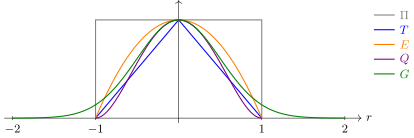
The kernels: rectangular , triangular , Epanechnikov , quartic — finite, on ; the Gaussian is positive everywhere. All five equal one at zero.
The recommendations are these. One can take the Gaussian kernel: its branches go off to plus and minus infinity, and every point of the training sample is guaranteed to make some nonzero contribution — all the terms in both the numerator and the denominator will be nonzero. Or, even better, the quartic kernel, a piece of a fourth-degree polynomial: it is smooth. The approximating function inherits the smoothness of the kernel: if the kernel is smooth, the function obtained by the Nadaraya–Watson formula will be smooth too, and we like smooth functions. The rectangular kernel is not very good: the function comes out piecewise constant, with jumps, and in many problems that is inconvenient.
Example (The window width and the type of kernel). Once upon a time there was a function that gave us the points of the sample, and we build three approximations with different window widths, .
The Gaussian kernel. If the window width is too small, we start chasing the noise: each value is obtained by averaging over a very narrow neighbourhood, over a few points. If the window is too wide, we really average over a fairly large part of the sample and oversmooth the function — in the limit, sending the window width to infinity, we get a constant. An optimum always exists: the window width affects the quality of the approximation very strongly and has to be chosen.
The triangular kernel is finite — nonzero only on the interval . With too small a window width, gaps appear: in some places the function cannot be computed, because in the Nadaraya–Watson formula both the numerator and the denominator have zero terms. If the window is taken wider, so that points are guaranteed to fall into it, there are no gaps. But the triangular kernel is piecewise linear, continuous and not smooth, and the Nadaraya–Watson formula gives a ratio of piecewise linear functions: the approximation is continuous but not smooth.
The rectangular kernel gives a function made of pieces, and again gaps with too small a window. With any finite kernel the window must be such that the neighbourhood of any point captures at least some objects of the training sample.
So:
- the kernel strongly affects the smoothness of the function and weakly affects the quality of the approximation;
- the window width strongly affects the quality of the approximation;
- a variable window width by the nearest neighbours:
where is the th neighbour of the object ;
- optimizing the window width — by cross-validation, exactly as for classification; one gets a plot with a characteristic minimum:
The problem of outliers
One more point is how to work with large outliers; I will talk about this in detail in another lecture. If two points with values and are added to a sample of a hundred points — note the scale: that is somewhere a floor above and a floor below — the approximation jerks towards these outliers. This can be used to identify outliers and effectively remove them from the sample. There is an algorithm that literally in one or two iterations finds such points and throws them out, and the approximation at the places of the outliers returns to where it ought to be.
Summary
Metric methods are, one could say, the simplest thing in machine learning, but even in them there is something to train: the number of nearest neighbours, the window width, the weights of the objects; objects can be thrown out, keeping prototypes. What I did not talk about and will not talk about is distance learning: how to introduce parameters into the metric itself and optimize them. Such problems are, on the whole, easily solved by the stochastic gradient method. An important insight we will return to in the next lectures: metric methods of the potential function type are a variety of linear classifier, where the amplitudes of the potentials serve as the parameters. And an interesting point is how to reduce a problem without features to a problem with features: measure the distances to prototypes. All the objects of the training sample can be taken as prototypes, reference objects, but that is inefficient; a selection can be made.
No comments yet
Be the first to share your thoughts.