August 30, 2026 · Lecture · LibreTimes
Machine Learning 1. Lecture 3. Neural Networks: Gradient Optimization Methods
Contents
- What this lecture is about
- A reminder: linear models of classification and regression
- Implementing Boolean functions with neurons
- The approximating power of neural networks
- The multilayer neural network
- The backpropagation method
- The problem: the gradient of a superposition of functions
- Recursive computation of the partial derivatives
- The BackProp algorithm
- Advantages and drawbacks
- Adaptive gradient methods
- Gradient explosion and gradient clipping
- Random switching off of neurons (Dropout)
- Activation functions
- Batch normalization
- Heuristics for the initial approximation
- Network pruning (Optimal Brain Damage)
- Seminar
What this lecture is about
Our course covers a large number of methods — one could say the classics of machine learning. Today people mostly talk about artificial intelligence built on neural networks; the other methods may be fading into the background, but they have not yet lost their relevance, so the course is a textbook one, covering all the methods. But I want to lead up to neural networks as soon as possible. In the second lecture we covered the linear model of a neuron — the linear classifier and linear regression. Today we will combine linear neurons into networks. The main goal is to understand how the main method of training neural networks, backpropagation, works, and to hang all sorts of heuristics on it, without which it does not work very well.
A reminder: linear models of classification and regression
The supervised learning problem: we are given a sample , the objects are vectors , that is, they are described by numerical features, and are the correct answers on the objects. If are discrete, it is a classification problem; if continuous, a regression problem. That does not matter to us now: we will consider a general method that solves both kinds of problems depending on the choice of the loss function.
The regression problem, . The linear model is the scalar product of the feature vector and the parameter vector . For generality I will add an activation function here — some transformation through which the linear model can be fitted to the distribution of the answers:
where is the error on the object, and is a unimodal function: is least squares, , and others.
The classification problem with two classes, . The model is : we are interested only in the sign. The loss function is a non-increasing function of the margin, smooth so that gradient methods can be applied:
for example is logistic regression, is SVM, and so on; we will study all these methods in turn. An amusing generalization: by choosing the loss function one can change the method. Once all these methods were invented from completely different considerations, heuristics and principles, and it turned out that all of it can be reduced to optimization, only with slightly different loss functions.
The next reminder: the linear model can be regarded as a model of how a nerve cell works — the McCulloch–Pitts neuron (1943):
where are the features of the object, the weights of the features, the activation threshold, and the activation function. Through its dendrites the neuron takes in charges, the weights are the share of the charge that passes into the cell, the sum is the total charge accumulated inside, and if it exceeds the activation threshold , the cell becomes excited and passes an impulse on. That is the fairy tale of how a neuron works. In reality neurons work quite differently: neurophysiology knows dozens of types of nerve cells that work in different ways. Nevertheless, this old, very first linear model of a neuron underlies practically all the neural network designs used in the most advanced tasks. To say that this resembles how the brain works is a real stretch — pulling an owl over a globe, as we say in Russian. But regarding a neural network as a universal approximator is a correct, purely mathematical statement of the problem. Let us talk about how rich a family of functions a neural network can implement.
Implementing Boolean functions with neurons
A single neuron can implement only a hyperplane. In classification it is a separating hyperplane that cuts the space into two half-spaces: one class lies on one side, the other on the other; the direction vector shows in which direction class lies.
Let the features be binary, zeros and ones, and the answers binary too. Then we are in the setting of functions of the algebra of logic, and any Boolean function can be implemented as a superposition of three elementary logical functions: AND, OR, NOT. If we show that these three functions are implemented by a linear neuron, that will prove that any Boolean function can be implemented by a superposition of neurons, that is, by a network.
Example (The functions AND, OR, NOT). For binary features :
Logical AND is a separating line in two-dimensional space that separates the point from the other points; OR is the same, only with the threshold ; the NOT operation amounts to putting a minus sign in front of the variable. Everything is implemented very easily.
Are there Boolean functions that cannot be implemented by a single linear neuron — do we really need to build superpositions? One example is enough, the textbook one: the exclusive OR function, XOR, . There is no way to separate two ones from two zeros with a single line.
Implementing AND, OR, NOT with neurons (slide); on the right, the separating lines on the unit square.
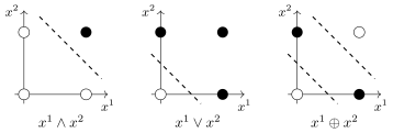
Black points have the value 1, white ones 0. AND and OR are separated by a single line, and . For XOR one line is not enough: the ones lie in the strip between two lines.
XOR can be implemented, and here are two examples that outline two completely different ways of implementing, with neural networks, functions more complex than linear ones.
Example (Two implementations of XOR). By adding a nonlinear feature (feature generation): we have the features and ; let us form their product and introduce it as a third feature. It turns out that this is enough:
By a network — a two-layer superposition of the functions AND, OR, NOT:
The first way extends the feature space: new features are synthesized, computed from the old ones. The implementation is not unique: clearly two ones can be separated from two zeros in different ways. The second way builds precisely a multilayer neural network.
A two-layer network for XOR and two ways of implementing it (slide).
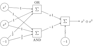
A two-layer network for XOR: the first layer computes OR (threshold ) and AND (threshold ), the second their difference with the threshold . The thresholds are weights of a constant input ; the activation functions are threshold ones.
Can any Boolean function be implemented with two layers? Yes. There is a theorem that any Boolean function can be written in disjunctive normal form — a disjunction of conjunctions of the original variables, some of which may be negated, and negation is simply a minus in front of the variable.
Proposition. Any Boolean function is implemented by a two-layer neural network: the conjunctions of the disjunctive normal form are the first layer, the disjunction over them is the second.
The conjunctive normal form, a conjunction over disjunctions, is obviously also implemented by a two-layer network. Moreover, there are algorithms that write out the disjunctive normal form for a Boolean function given as a table — for each combination of inputs, the output is given. That is, literally from a sample, from a table, one can build a two-layer neural network.
The approximating power of neural networks
It might seem that perhaps two-layer networks are enough to approximate an arbitrary function? Let me list a few well-known mathematical facts.
- A two-layer network implements an arbitrary Boolean function — I have already said this.
- Geometrically: each linear neuron splits the space by a hyperplane into two half-spaces in its own way. If we build a second layer, a linear combination of these neurons, then, as is easy to prove, some polyhedral region is singled out — in general not necessarily connected and not necessarily convex.
- Any continuous function can be approximated with any accuracy by a two-layer neural network. To increase the accuracy, we simply increase the number of faces of the polyhedron, that is, the number of linear neurons.
This mathematical result slowed down the development of deep neural networks somewhat in its time. On the one hand, mathematics seems to say that two layers are enough. On the other hand, biological evolution suggests that the brains of humans and animals do have many layers. The number of layers can be estimated like this: divide a creature's reaction time to a stimulus by the time it takes an impulse to pass through one neuron. Both can be measured in experiments, and such estimates have been made: not many, 10, 15, 20 — but that is still a deep network, not two layers. So nature arranges deep neural networks in brains for a reason, and not only in humans but in much more primitive animals as well.
There is another theorem, Cybenko's — he is an American scientist, despite his Slavic surname.
Definition (Sigmoid). A function is a sigmoid if and .
What exactly this function looks like is not so important: what matters is that it tends to zero and to one at minus and plus infinity.
Theorem (Cybenko, the universal approximation theorem, 1989). If is a continuous sigmoid, then for any function continuous on there are parameter values , , , such that the two-layer network
uniformly approximates with any accuracy :
That is, there exist a number of neurons in the network, coefficients in the second layer and coefficients in the first layer such that the network approximates an arbitrary given function with any given accuracy. We will not go into the details of how the theorem is proved; there are many different theorems on this subject. What is important to remember is that a neural network is a universal approximator of smooth functions, and that two layers seem to be enough for approximation, which means three or four are certainly enough.
The multilayer neural network
Now we will consider, in general, a deep network with a large number of layers . The notation is important: you will have to peek at it or write it down on a piece of paper.
Definition (A fully connected neural network with layers). Network architecture: is the number of neurons in the th layer, ;
- is the feature vector at the input of the network, ;
- is the feature vector at the output of the th layer, ;
- is the output vector of the network, ;
- is the weight matrix of the th layer, of size .
By default the zeroth feature is the constant . This is done so that everything can be written simply as a scalar product and we can forget that is some activation threshold: we introduce an additional constant feature and increase the dimension of the scalar product by one. It is just a form of notation; it is customary and more convenient.
At the input is the input layer, the features themselves. Having computed some number of neurons over the input features and written the results as a vector, we get a new feature description ; the same happens in the second layer, the third and so on. Remember: is the vector of features computed by the th layer; these are no longer the original features. The last layer is called the output layer. The established terminology is: one input layer, one output layer, and all the others are called hidden. Nobody hid them from anyone — they are hidden simply because they are between the input and the output. We set all the dimensions in advance, and by setting them we set the architecture of the network. The dimension of the output vector may be one if the network predicts a single output; many outputs are needed, for example, for multiclass classification. In the weight the superscript is the layer number, is the input number, the output number: each weight is an edge connecting the th neuron of layer with the th neuron of layer . And the outputs of the network we will also denote : this is the model we are building, and is the index of a coordinate of the output vector.
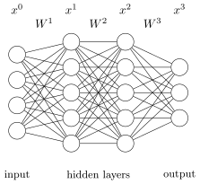
A fully connected network with layers: the input vector , the hidden layers , , the output vector ; the matrix connects every neuron of layer with every neuron of layer . The constant inputs are not drawn.
The backpropagation method
The problem: the gradient of a superposition of functions
Now we will play with this notation. The task is to understand how to train this contraption by a gradient method. In the previous lecture there was the stochastic gradient method for a single linear model, and it is not hard to generalize it to a neural network: we only need to be able to compute the gradient of the loss with respect to the whole set of weights of the network.
Definition (The stochastic gradient method SG). Minimizing the mean loss on the training sample: .
Input: the sample ; the learning rate ; the parameter . Output: the weight vector of all the layers .
- Initialize the weights and the current estimate .
- Repeat:
- pick an object from (for example, at random);
- compute the loss ;
- gradient step: ;
- estimate the value of the functional: ;
- until the value of and/or the weights stabilize.
The main thing in this algorithm is the gradient step. We accumulate the functional as an exponential moving average to take it into account in the stopping criterion. But often the process is stopped simply when a given number of iterations is reached: we will do 1000 iterations, and even if we converged after the 278th, we will do all the rest. Stopping criteria are always heuristics, not only in machine learning but in optimization methods generally.
The most interesting and most important thing is how to find the gradient over this crazy number of weights, which moreover sit in different layers of the network. What is the difficulty? It is precisely what held back the development of this science for a long time: backpropagation was invented only in 1986, and before that networks were mostly built layer by layer. One layer is built, it gives a new feature description; we take it as features, build the next linear classifier, and so on, layer by layer. This is an outdated approach.
Think about it: the gradient vector is the partial derivatives with respect to all the parameters of the network. To compute one partial derivative takes a number of operations proportional to the complexity of the whole network: computing the network itself and computing its derivative with respect to a parameter are comparable. And a partial derivative is taken with respect to each parameter in turn, so in all it comes to the order of operations. These simple considerations held everything back for a long time: quadratic complexity on hardware before the eighties allowed only very simple networks to be trained. Then a way was invented to compute the gradient of a superposition of functions in a number of operations that is not quadratic but linear in the number of coefficients. That is backpropagation, and its main trick is computational efficiency. It turned out that if one carefully differentiates a superposition of functions and remembers the right intermediate computations, the computation can be organized an order of magnitude more efficiently.
Computing the network for an input vector , recursively layer by layer. We start with the vector of original features and then go layer by layer: take the features at the output of the previous layer, sum them with the weights connecting layer with layer , get the outputs of the summators , and apply the activation functions to them:
Usually the activation function is certainly the same for all the neurons of one layer; sometimes different layers are assigned different functions, sometimes there is one throughout the network. For generality I write , leaving each neuron the possibility of its own. What matters is that the function is fixed, has no parameters, and can be differentiated with respect to its single scalar argument. In matrix notation the same thing looks much more elegant, and that is how it is most often written in papers and popular blogs:
where the matrix is multiplied by the vector , and the same activation function is applied to all the elements of the resulting vector.
The loss on the object is the very function that will have to be differentiated at each step of the stochastic gradient. I will use the general notation — we need to understand how to solve the problem for an arbitrary loss function — and, as an example, glance at what happens in least squares:
We need the partial derivative with respect to the coefficient , which connects the th neuron of layer with the th neuron of layer . By the chain rule we differentiate through the intermediate variable :
This is a very important technique. Now let us write out all these partial derivatives separately and understand how to compute them efficiently.
Recursive computation of the partial derivatives
First we find the partial derivatives of the loss, whatever it may be, with respect to the coordinates of the vector at the very last layer, . For the quadratic loss we immediately get a very simple result:
— this is nothing other than the error of the output layer: the difference that stood under the square is all that remained after differentiation. The deviation of the th output of the network from the correct value on the th object. I deliberately say everything in words so that you keep checking the indices against their meaning.
Now let us go through the layers backwards and, for an arbitrary layer, compute the partial derivatives recursively, from right to left, . Usually we compute the network from left to right: on the object we reached the end and computed the errors . Now let us go through the network from right to left — hence the name, the method of backpropagation of errors. We express the derivative with respect to through the derivatives in the th layer — this is simply the chain rule: we sum over all the neurons of the th layer the derivative that by the inductive assumption has already been computed, multiplied by the derivative of the activation function at the same point where we computed the function itself on the forward pass, and by the weight:
The derivatives with respect to the outputs of the th layer we denote and formally call the errors of the hidden layer. For the penultimate layer, are the errors on the last layer, which we already know. Knowing them, we use this formula to compute for layer , and then layer by layer from right to left, in decreasing .
Remark (Why «errors»). The derivative of the loss with respect to the outputs of the last layer turned out to be the error — but only for the quadratic loss; for other functions it is something like an error, and calling it that is already a bit of a stretch. And on the hidden layers we call the partial derivative an error purely formally: it is no error at all, just a convenient name for an auxiliary quantity we compute in each neuron of each layer. So when people say «backpropagation of errors», it is these that propagate. If we take another loss function, the changes are minimal: only the formula for changes.
The activation function and its derivative are computed at the same point . We of course know the derivatives of the activation functions: we choose the activation functions ourselves, whatever smooth functions we like. It makes sense to store not but straight away — the value of the derivative of the activation function at the point given by the summator.
Let us realise that the recursive formula we obtained is written as if the network were run backwards: knowing on the next layer, we compute on the previous one, multiplying them by . The summator, which in the network architecture worked from left to right, works from right to left in backpropagation.
Now, having the partial derivatives of with respect to all , it is easy to find the gradient with respect to the weight vector:
Three types of variables travel around the network: , and . The values of we compute when going from left to right, and we must remember them across the whole network, because they will be needed on the backward pass; is also needed for the gradient. I said at first that need not be remembered — it is enough to pass them from the next layer to the previous one — but no: the partial derivatives needed in the gradient step depend on them, so , and are all stored. Not much of a memory cost: computational efficiency has to be paid for with RAM to store intermediate computations, but we gain a lot in speed.
The BackProp algorithm
Definition (The backpropagation algorithm BackProp). Input: the sample , the architecture , the parameters , . Output: the weight vector of all the layers .
- Initialize the weights .
- Repeat:
- pick an object from (for example, at random);
- forward pass: for all ,
- computing the errors: for all ;
- backward pass: for all ,
- gradient step: for all , ,
- until the value of and/or the weights stabilize.
The logic of the stochastic gradient stays the same: pick an object at random, and then three passes — forward, backward and the gradient step. Allow me to introduce: the backpropagation method, back propagation, which is used to train neural networks, including deep ones and of any architecture.
What does «architecture» mean? It is not only the number of layers and the number of neurons in each layer. One can say that each neuron depends not on all the neurons of the previous layer but only on some subset of them; such networks are called not fully connected. But that is the same as setting some coefficients to zero. If we know for certain that a coefficient is zero and is not used in the network, it simply need not be computed in the algorithm: it is taken out of the loop, and that is all. We wrote the algorithm for a fully connected network, where each neuron of the next layer depends on all the outputs of the previous one, but that is not at all necessary. Many types of networks, convolutional ones for example, specify exactly which neurons of the previous layer each neuron depends on, and there are very few nonzero connections there: the network is highly sparse. This in no way hinders computation by the BackProp algorithm: it adapts very easily to any neural network architecture; the loops simply run not over all variables but only over the nonzero weights.
Advantages and drawbacks
The cost can be seen from the algorithm: the forward pass, the backward pass and the gradient step all require a number of operations linear in the number of weights. That is the main miracle.
Advantages:
- the time to compute the gradient is instead of — thanks to clever differentiation of the superposition of functions and to storing the intermediate quantities;
- generalization to any architectures, any activation functions and any loss functions ;
- the possibility of dynamic (streaming) learning: the sample keeps growing, a new object arrives — we immediately pass it through the algorithm; after all, inside the loop we compute for one individual object each time anyway. Objects can be run in random order, or in their natural order if the problem is dynamic and the objects arrive in time: this is how one learns on signals and time series, and how one learns to play computer games;
- the possibility of parallelization: all the sums can be computed in parallel if such processors are available. Graphics cards, invented to draw thousands of little triangles on the screen at once, were adapted to compute thousands of neurons at once.
Drawbacks — all the same ones characteristic of stochastic gradient:
- slow convergence;
- getting stuck in local extrema;
- paralysis — vanishing gradients due to the horizontal asymptotes of the activation functions: you land at a point of the coefficient space where the derivative of the loss is close to zero because the derivative of the activation function is close to zero. The gradient step is too small, and it is very hard to get out of such an unlucky place;
- gradient explosions due to the ravine-like landscape of the criterion;
- overfitting: each neuron is a linear model, and linear models suffer from multicollinearity, so some regularization must be applied to each neuron;
- choosing a set of heuristics is an art.
Experience has accumulated over the decades, and in good implementations all of this is already built in under the hood. But one has to understand that this is not trivial: people did not at once work out which set of heuristics to put into stochastic gradient to make it converge fast. Let me add to the heuristics I told you about last time.
Remark (Fast differentiation of arbitrary superpositions). After the lecture someone asked: early deep learning libraries seem to have simply computed by the formulas, while modern ones build a backpropagation graph — is this an improvement of the algorithm or just a convenience? It is a generalization. I told you how to differentiate a fairly rigidly structured superposition of functions: a fully connected network, neurons, activation functions — that is, I imposed restrictions on the structure of the superposition. But if you simply write out a superposition of some functions, linear, nonlinear, scalar activations and so on, the same can in principle be done with it. This requires so-called fast, automatic differentiation: a superposition of functions written as program code has to be literally differentiated automatically to get other program code that computes the derivatives. Modern libraries do something in this spirit, so that one can write down not only such a neural network but something stranger: even in as general a setting as here, the restrictions may turn out to be significant for some architectures. A rather impressive implementation of analytic differentiation of superpositions of functions of fairly arbitrary form has been done there.
Adaptive gradient methods
Let me remind you of a slide from the last lecture: two very nice techniques that really do speed up convergence a lot.
Definition (Momentum and the accelerated gradient). Momentum — the exponential moving average of the gradient over the last iterations [B. T. Polyak, 1964]:
NAG (Nesterov's accelerated gradient) — stochastic gradient with momentum [Yu. E. Nesterov, 1983]:
Momentum averages the gradient on the current object with what has been accumulated so far in , and the averaged gradient shows a more correct, more stable direction in which the functional decreases. The accelerated gradient is when the gradient is computed at a more correct point: we already know where we are going to move, and that is where it should be taken.
But there are other interesting inventions too. It was noticed that when a neural network has a huge number of parameters — millions or even billions — the rate of convergence may differ across coefficients: along some we converge fast, along others we get stuck. Can the gradient step be equalized so that the speed is the same along all coordinates?
Definition (RMSProp). RMSProp (running mean square) — equalizing the rates of change of the weights by a moving average over iterations; it speeds up learning for the weights that have so far changed little:
where and are coordinatewise multiplication and division of vectors.
Everything here is written in vector notation. The circle with a dot is coordinatewise multiplication of two vectors: the first coordinate of the first vector is multiplied by the first coordinate of the second, and so on for all coordinates. So is the exponential moving average of the vector of squared partial derivatives of the loss with respect to all parameters. The root of the averaged squares is something like the root mean square for each coordinate of the gradient vector, and we divide each coordinate of the gradient by this norm. In this way we say: let the rate of change of the vector be roughly the same along all coordinates. It seems that we are no longer moving in the direction of the antigradient: having divided it coordinatewise by another vector, we have moved off somewhere to the side. But we go in such a way as not to get stuck in any coordinate and to move along all coordinates at equal speeds — and this turned out to be a very successful technique that speeds up convergence.
The next variant answers the question of where to get the gradient step : we would like to choose it more or less automatically. Last time we talked about the Levenberg–Marquardt method, where the step can be taken as one divided by the second partial derivative with respect to the corresponding parameter. But one does not always want to compute second derivatives either.
Definition (AdaDelta). AdaDelta (adaptive learning rate) — double normalization of the weight increments, after which one can take :
is computed as in RMSProp; is the moving average of the squares of the increments themselves. The gradient is normalized twice: by the norm of the gradient and by the speed of progress. Such a step no longer has to be adapted: it can be set once, even set to one, and the process will itself choose the gradient steps from iteration to iteration. You see: with a few heuristics — the exponential moving average, normalizing the gradient, double normalization — we are in fact no longer following a gradient method. We go in a direction in which the function decreases, but not the steepest in the sense of derivatives, rather the steepest in the sense that we will move there faster.
Dozens of modifications of these methods have been invented. Adaptive momentum, Adam, combines momentum and RMSProp and requires a calibration that adapts the size of the gradient step: the steps are large in the first iterations, when we have not yet really understood where we are going, and smaller and more careful as we approach the optimum. This can also be combined with Nesterov's accelerated gradient.
Definition (Adam and Nadam). Adam (adaptive momentum) = momentum + RMSProp:
The calibration , increases , in the first iterations, where is the iteration number; , , .
Nadam (Nesterov-accelerated adaptive momentum): the same formulas for , , , , and
The heuristics combine with each other in various ways and give rise to a whole family of gradient methods. Which of them works faster in all situations is impossible to say. On the internet you can find a huge number of animations built on all sorts of functionals; these are all demonstration examples, but even they show that there is no method that wins on every landscape of the function being optimized: one is faster here, another there. Holy wars break out: one says you should always use Adam, another AdaGrad or something else. These are heuristics, and it is impossible to prove a theorem that one method is always faster than another; there is no unambiguously best choice. They can always be combined: if one method has started to work slowly, switch to another, or even change the method at random in the hope that another will converge faster. With such switching one can adapt to the landscape of the function being optimized.
Gradient explosion and gradient clipping
Another problem is gradient explosion (gradient exploding), and there is a simple heuristic for it. The cause is the ravine-like landscape of the criterion being optimized. Suppose we are next to a narrow ravine that leads in the direction of decrease. We went down the ravine a little, and the next gradient step threw us onto the opposite side, which turned out to be very steep. The next step, computed from a huge gradient, carries the process off to some distant point — and you have to start all over again.
Definition (Gradient clipping). If , then , where is the gradient vector and is the threshold.
If the norm of the gradient vector has suddenly become larger than the given threshold, we simply divide the gradient by its norm and multiply by the maximum allowed value of the norm. The direction stays the same, but the shift along the antigradient in one step cannot exceed the threshold . Such a heuristic in principle solves this problem.
Of course, one should also think about how to construct the functional so that there are no such sharp cliffs, how to make it smoother; we will talk about that later. One such technique was found when deep neural networks were being built for images: in 2015 networks with so-called skip connections appeared. It turned out that they improve the landscape of the criterion being optimized very nicely, making the functional much smoother and free of local extrema. Such effects are either absent there or occur much less often. It is not at all obvious why a change in the network architecture can smooth the landscape so that neither getting stuck in local minima nor gradient explosion from sharp jumps of the functional occurs. But the problem still cannot be solved once and for all, and the gradient clipping heuristic is, I believe, simply built in everywhere; if need be, one can tweak the additional parameter .
Remark (How skip connections work). Someone asked about a paper that studied how the gradient passes through a skip connection: it turned out that it does not pass straight through but flows along all possible paths, and everything is more complicated than it seems at first sight. There are several explanations of how skip connections work and why a network with them is more stable; this is one of them. Another is what I have already said: papers have pictures of the landscape of the functional being optimized, and one can see how skip connections smooth it and rid it of local extrema. My interpretation is very simple. A skip connection says: one or several layers between the points it connects are a small addition to the network that was already there. Mostly the previous network does the work, and these layers are needed only to correct it slightly; let the coefficients there be small. When everything is trained together, the subsequent layers learn small corrections and do not overfit. More on this next semester, in the lectures on deep neural networks and convolutional networks for images.
Random switching off of neurons (Dropout)
Another good technique is called dropout; I tried to translate it into Russian as «the method of random switching off of neurons». In its time it was very popular, less so now, but it still turns up from time to time.
The idea came from neurophysiology. Biological neurons switch off from time to time and rest — this is called relaxation: at that moment they can neither learn nor work. But the network as a whole keeps functioning reliably; it is insensitive to such switch-offs. How can this be done with artificial neural networks? They have to be trained so that the weights of the whole network get used to the idea that some of the neurons may be relaxing and not working.
The idea is very simple. When taking a gradient step on the th object, that is, training all the coefficients of the network, let us switch off some random subset of neurons: set their outputs to zero; they will not be used in this gradient step. At the next step we again choose a random subset, and so at each step a random subset of neurons of its own is relaxing. The network gets used to someone always sleeping in it at random — and there may be quite a lot of sleepers. The network learns to work when, say, 15% of its neurons, nobody knows which, are switched off, and to do so in such a way that it does not affect the result.
Definition (Dropout). Training stage: when taking the gradient step , switch off the th neuron of the th layer with probability :
Application stage: switch on all the neurons, but with a correction:
What will the network learn from this? Redundancy: neurons will start duplicating each other's work. As neurophysiologists say, an impulse never travels alone from one neuron to another: a wave of excitation goes, hundreds or even thousands of neurons transmit the same impulse synchronously from one place to another. It is a reliable stream, and if some of the neurons drop out of it, the result still reaches its destination. Here the idea is roughly the same. We generate a random variable that with probability zeroes the neuron's output: the neuron did not fire, output zero, slept and rested, and nevertheless the network as a whole must keep working correctly. The only nuance: if a certain share of the neurons is switched off, the total output is smaller by that share. So at the application stage the output has to be multiplied by the correcting factor , and that is slightly inconvenient when computing on new objects.
People learned to deal with this very simply — inverted dropout. Apply the factor right at the training stage: because of the random switch-offs the output decreases slightly, and we immediately divide it by , so it increases by the same factor. Then at the application stage neither modifications nor knowledge of are needed: the ordinary formula for computing the neural network works.
Definition (Inverted Dropout). Training stage:
Application stage: .
Why does dropout work, after all?
- Voting. A theorem was proved that dropout is in effect a simple vote over an astronomical number of networks: over all possible ways of switching off, say, 15% of millions of parameters. There are probably more such configurations than atoms in the Universe. The result is purely formal and non-constructive: it gives an interpretation but is useless for computation.
- Regularization. We reduce the opportunities for overfitting by telling the neurons: do not fit yourselves to each other, do not compensate for each other's errors, let each one solve the original problem. Different parts of the network are forced to solve the same original problem, and the network becomes a little more like a composition of different algorithms dissolved in each other: simpler architectures together form a more complex one, but act, as it were, separately.
Regularization can also be inserted explicitly. Last time we said that regularization is a remedy against multicollinearity. Each neuron is a linear model, multicollinearity can arise in it, so it is very useful to add regularization, which will press the coefficient vectors towards zero and keep them from running off to plus or minus infinity:
There it is, the factor at slightly less than one: that is the decay, weight decay, or, as people also say, ridge, shrinking the vector . The modification of the gradient step is not much of a complication: here, a correction factor slightly less than one in front of the vector ; there, randomly switched-off neurons and division by . It is an edit to one line of code, and both regularizations are easy to implement and even to combine: the gradient is then computed over the network with switched-off neurons.
Activation functions
Another important point is how to choose activation functions. I have already said: if an activation function has horizontal asymptotes, like the sigmoid or the hyperbolic tangent , this may lead to vanishing gradients, to network paralysis. When the arguments reach the horizontal asymptotes, the derivatives are close to zero, the gradient step is very small, and if you get there, it is hard to get out.
How to fight this? Unexpectedly, an activation function made of two linear pieces turned out to be a very good solution — the rectified linear unit. On the negative side the derivative is simply zero, on the positive side a constant one; this also simplifies all the formulas and speeds up computation.


Activation functions: the sigmoid and the hyperbolic tangent have two horizontal asymptotes (dashed), softplus and ReLU have one, on the left; PReLU (here ) has no horizontal asymptotes.
It turns out that if the horizontal asymptote is not on both sides but only on one, the network does not fall into paralysis. Softplus is built this way too: it does have a branch without a horizontal asymptote. A huge number of activation functions have been invented; everything has been tried. In recent years a combination of ReLU and sigmoids has been used. A sigmoid is needed, for example, when the output of a classification network has to be turned into probabilities from zero to one: there is no getting around it there. But only in those layers whose output is interpreted as a probability — there one can use a sigmoid or some SoftMax. In the bulk of the layers in recent years ReLU, the rectified linear unit, is used, or leaky ReLU when one does not want completely zero derivatives: a piecewise linear function with a kink. It is not smooth, but that has practically no effect on the gradient step, so such functions can be used too.
Batch normalization
Normalization deserves a separate lecture: all sorts of things are normalized in training neural networks. Here I will show batch normalization, a very important technique.
Neural networks are trained on big data, and the trouble may be that one feature is measured in numbers close to zero, another in numbers of the order of millions, a third ranges from minus a million to plus a million. Clearly all features have to be centred and normalized: vectors normalized somewhere around zero are much more convenient to work with, it is computationally more stable and does not lead to accumulation of errors. But normalizing is hard: how do you normalize over the whole sample if there are millions of objects? Let us cut the sample into batches, say of 1000 objects. Looking at 1000 objects, one can already compute the mean and variance of each feature and normalize it. But here is the trouble: after we have normalized the features on one batch and moved on to another, the normalizations there will be slightly different. By the law of large numbers they will be similar, but the means and variances will change slightly. On the one hand, normalization is needed to make the computation more stable; on the other, the different normalizations have somehow to be brought to a single one.
Definition (Batch normalization). is a batch (mini-batch) of data, are the vectors of the objects at the output of the th layer.
Normalizing each th component of the vector over the batch:
Compensation: is a linear layer; the parameters and are tuned by BackProp.
The values at the output of the th neuron of the th layer are averaged over the batch — here is the mean, here is the variance; we subtract the mean and divide by the root of the variance. But the normalizations are slightly different for different batches. To even this out, we add a linear layer with tunable coefficients and — also a linear neuron, without any activation function — and this linear transformation is tuned together with the whole network by back propagation. The idea turned out to be very successful because it is adaptive: the composition of objects in different batches may turn out quite different; the split of the sample into batches need not be representative or random. Even though the normalization is different in each batch, the overall alignment of these normalizations leads to very stable training. A simple technique, it would seem, just normalization, yet it makes the training process computationally stable.
Heuristics for the initial approximation
I showed heuristics for the initial approximation in the last lecture, but there are a few new thoughts here.
- Not a new thought: draw the weights from distributions reasonably close to zero — and then apply corrections that equalize the variances of the outputs and gradients in different layers.
- Layer-by-layer training of neurons as linear models — on a random subsample, on a random subset of inputs, or from different random initial approximations; this ensures that the neurons differ. As I have already said, layer-by-layer training was popular in the seventies and early eighties, before back propagation appeared, and it was used later too. It is a very simple way: we train the first layer as different linear models, make them diverse but such that they all solve the same original problem; then we represent the outputs of these models as one feature vector and do the same over it, and so on. Such training is reasonably stable, though not very good in itself, but it is a very good start from which to launch back propagation.
- Initialization with the weights of a pretrained model.
- Initialization with a random orthogonal basis.
A huge number of these techniques have been invented; we will not go deep.
Network pruning (Optimal Brain Damage)
Finally, one more interesting technique with a funny name — optimal brain damage. Let us zero out weights that are not very useful. How do we determine the usefulness of the model's parameters for the problem of minimizing the criterion ?
Let us write the second-order expansion of the criterion — the multivariate Taylor formula — in a small neighbourhood of the point . Why is there no first-order term? Because we expand at the optimum point: imagine that is a minimum point we have already reached. In its neighbourhood the functional behaves roughly as a quadratic form in the shift :
is the Hessian, a matrix of size .
The heuristic is exactly the same as in the Levenberg–Marquardt method: we assume that the Hessian is approximately diagonal, depends only on the second partial derivatives, and the mixed derivatives are zero. Then there are no mixed terms in the quadratic form:
And the question of what happens if we zero the weight , that is, add to it, has a very easy answer. The contribution of a single parameter to the quadratic form, and hence to the functional itself, is multiplied by the second partial derivative, and .
Definition (The salience of a weight). The salience of the weight is the change in the functional when it is zeroed:
The English word salience means, on the one hand, significance and, on the other, prominence, a bulging out. Here it is literally the degree of convexity of the quadratic form along the given coordinate: how convex is along the coordinate at the minimum point. If the salience is large, the quadratic form depends substantially on this variable, and it must not be zeroed. If the contribution is small, the weight can be zeroed, turning the fully connected network into a not fully connected one and getting rid of unnecessary connections.
Definition (Network pruning OBD).
- In BackProp, compute the second derivatives .
- If the process of minimizing has reached a minimum, then
- in each layer, sort the weights by decreasing ;
- remove the connections with the smallest salience;
- run BackProp again.
- If or has become substantially worse, restore the connections removed last and stop.
Yann LeCun, John Denker, Sara Solla. Optimal Brain Damage. 1989.
This can be done in a loop. We did a few iterations of back propagation, computed the saliences of all coefficients, zeroed the smallest. After zeroing, the network is under stress: part of its connections have been cut out, it becomes a bit crazy and starts working slightly worse. But a few more iterations — and it returns to normal, and this normal may turn out even better, because throwing out unnecessary connections reduces overfitting: this too is a kind of regularization. Again we reached a minimum, computed the saliences, zeroed the unneeded ones — the network jerked towards psychosis again, a few more iterations, and it normalized again. An interesting result: the network can converge to a sparse state that works even better than the fully connected network.
The method is fairly old, the late eighties, and in its time it was used very actively; it was considered the state of the art in training neural networks. Then people learned to do many other regularizations, to combine dropout with and regularization, skip connections appeared, and the pruning method fell out of favour; it is little used now. But it is useful, first, for sparsifying a network, and second, it can even be used to identify redundant features: sum the saliences of all the weights connected to a feature,
and cut out uninformative features. In the same way the number of neurons can be reduced: sum the saliences over all the connections of a given neuron and, if the sum is small, switch it off from the network. In this way the network can be gradually simplified.
Remark (How many connections to remove). Someone asked how many connections are removed at each iteration and how many can be removed in all. It depends on how the complexity of the problem relates to the complexity of the architecture taken for it. If you took a highly redundant network and the problem is simple, you can remove even 99% of the connections: a sparse network sufficient to solve the problem will remain. If the problem is complex, you may manage to zero perhaps 10% or half — it varies.
Someone also asked about interpretation: if the method showed that some data are unimportant, can they then not be collected? Yes, if by data we mean features: feature selection can be arranged this way. If it turns out that, say, 50 features out of a thousand are informative and sufficient to solve the problem — there you have an example of 95% of the features not needing to be collected.
No comments yet
Be the first to share your thoughts.