August 30, 2026 · Lecture · LibreTimes
Machine Learning 1. Lecture 2. Stochastic Gradient and the Linear Classifier
Contents
- What this lecture is about
- Four steps: regression, binary and multiclass classification
- The separating surface and the margin
- Error analysis by margins
- The multiclass case
- Continuous approximations of the threshold loss
- The linear classifier is a model of a neuron
- The stochastic gradient method
- Gradient descent
- The algorithm
- Recursive estimation of the functional
- Speeding up convergence: momentum and the accelerated gradient
- Heuristics of the stochastic gradient method
- Weight initialization
- The order in which objects are presented
- Choosing the gradient step
- Advantages and drawbacks of the SG method
- Multicollinearity and regularization
- The probabilistic statement of the classification problem
- Likelihood and the approximated empirical risk
- The probabilistic meaning of regularization
- The Gaussian and Laplace priors
- Seminar
What this lecture is about
A dense lecture. Today: linear models of classification and regression and the stochastic gradient method; with these I will lead you up to the problem statements and methods used in training neural networks, and we will reach the networks themselves in the next lecture. At the end there will be one more important topic — the probabilistic statement of the classification problem and the probabilistic meaning of regularization.
Four steps: regression, binary and multiclass classification
In the previous lecture I showed you the method of least squares, and we looked at how linear, and in particular polynomial, regression works. Let us once more bring all this into a scheme of four steps and then extend it to classification.
The regression problem. We are given a training sample — «object — answer» pairs , the answers are real numbers, . We solve it like this:
- Fix the model — here the linear regression model, a linear combination of all features with coefficients :
Get used to writing it as a scalar product: from now on I will mostly use this vector notation.
- Fix the loss function — let it be quadratic, so that we get the method of least squares.
- Reduce learning to optimization: sum the losses over all the objects of the training sample and fit the parameter vector so that on the given objects the model gives answers as close to the correct ones as possible:
- Check on test data. For machine learning, optimization is only a tool. We must build a model that has predictive power, or generalization ability — people say it differently. We check this on a test sample, on data not used in training at all: the mean loss on it must also be adequate, small enough.
The binary classification problem. Now the same scheme for classification; I deliberately made two very similar slides. The answers are classes, and there are two classes: . The problem is called binary because we make a discrete «yes» or «no» decision: treat or not treat, grant a loan or not, is there oil in a region or not. As we saw in the previous lecture, there are very many such applied problems.
The model is again a scalar product, but now we are interested not in its value, only in its sign:
If the scalar product is greater than zero, the object goes to class ; if less, to class .
How should the loss function be built? It would seem nothing could be simpler: take the condition that the classifier errs. The classifier returns , the correct answer is also . If their product is negative, they have different signs, that is, the answer the classifier gives does not coincide with the correct answer . The function does not change the sign of its argument, so the scalar product itself can be substituted for , and an amusing and very useful construction arises:
What is its geometric meaning? The equation defines a hyperplane in with direction vector , which divides the space into two half-spaces. In the positive direction, where points, lie the objects of class ; in the opposite half, the objects of class . The quantity shows, roughly speaking, the signed distance from the object to the separating hyperplane. If is an object of class and the angle between it and is acute, it has landed in the right half of the space, and the product is greater than zero. If it is less than zero, the object has landed in the wrong half, and an error has occurred on it.
Definition (Margin). The quantity is called the margin of the object : it shows how far the object is from the separating hyperplane, and whether it is on the wrong side. The smaller the margin, the worse; if and only if the classifier errs on .
The threshold loss — these square brackets — is unpleasant because its values are discrete. If we build the functional as a sum of discrete losses, we get a discrete-valued criterion, very inconvenient for optimization. So we will minimize not it but an upper bound on it: take a continuous, or better a smooth, function that bounds the threshold one from above:
Then we approximately minimize the number of errors on the training sample, and we will be able to get a fairly decent vector this way. Here is a very important principle, which can now be called the dominant one in classification theory — the principle of approximating the threshold loss function. We have not only made the problem nicer for numerical methods: in this way we can also penalize an object for approaching the separating hyperplane; more on that a bit later. The fourth step, checking on test data, we of course do not forget.
The multiclass classification problem. What if there are many classes? Now is a finite set of classes, in general more than two. We would still like to keep the model linear. This construction helps: again we compute a scalar product, but each class has its own direction vector, and we assign the object to the class for which the scalar product is largest:
How is this to be interpreted? Each vector says: the objects of my class lie in that direction, and the farther you go there, the more objects of my class there are. Since each class has its own preferred direction, somewhere at the junction the models have to sort things out among themselves and come to an agreement; most likely there will be errors there, and we need a criterion that makes the errors as few as possible.
The loss function is again binary: if we guessed the class wrong, we must be penalized. But an object of class can be confused with different classes, and confusing it with one class is not as bad as with ten. So it is proposed to sum the errors over all the wrong classes : the scalar product should have been the largest among all classes, and the number of classes for which it turned out smaller is the loss. The binary loss is still inconvenient, but we already know how to deal with it: turn the logical condition into a margin, now for each pair «correct class — wrong class »:
The larger it is, the better; if the scalar product for the correct class is larger than for all the others, all such margins are positive and there is no error on the object. The learning method is still empirical risk minimization, only one more sum appears: over all the objects of the sample and, for each object, over all the wrong classes:
Here we use the «one against one» principle: all classes are compared with each other pairwise, and each pair of classes is handled as a binary classification. There are other strategies for multiclass classification too.
In supervised learning problems, in particular regression and classification, we follow this scheme all the time: we look at what data we have; we understand what model we are building; we formalize learning as an optimization problem; we check the model on test data. This is a fundamentally important scheme, and we will use it throughout the course.
The separating surface and the margin
Does it matter so much for this scheme that the model is linear? Of course not: that was just an illustration to make things easier for you. Nonlinear separating surfaces in classification? Easy: the scalar product will have to be replaced by some other function of the object and the parameter vector. And the vector is then not at all obliged to have the same dimension as — it all depends on how the model is built.
Definition (Margin-based classifier). A binary margin-based classifier: , , where is the separating (discriminant) function, a parametric family of functions; is the separating surface between the classes;
is the margin of the object ; the model errs on .
If we have written out the discriminant function and found the parameter vector , we know what the separating surface between the classes looks like: it is the locus of points of the object space where . The margin is still a kind of signed distance to the separating surface, but now the surface can be curved, anything at all, depending on how the function is defined. The meaning is the same: the margin is negative if and only if the algorithm makes an error on the object.
Error analysis by margins
Most classification methods rest on introducing something like a discriminant function, and here is a very useful plot that can tell a lot about how well the problem has been solved. On the training sample, and on the test one too — as long as the correct answer is known — we can compute the margins of all objects, sort them in increasing order and look at the result as a plot.
Objects sorted by increasing margin (slide): noise, borderline and reliable.
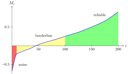
The margins of the sample's objects sorted in increasing order. On the left, in red, the noise objects with a large negative margin; in the middle, the borderline ones, near zero; on the right, those classified reliably.
On the right are the objects classified very reliably: they lie deep inside their class, all is well with them. Where the margin is negative there are errors, but errors differ. Errors along the boundary between classes may happen under the influence of random factors. But objects with a large negative margin most likely fit our classification model very badly. This may be due to noise: for example, some features were measured completely wrong, or even the answer was mixed up. There can be very many reasons why an object flies off into the noise region, and it is always useful to look at this plot. It is even more useful to overlay the same plot for the test sample: if on the test the curve shifts too far to the right, that is, the margins there are much worse, that is the effect of overfitting.
The multiclass case
In multiclass classification a separate discriminant function has to be built for each class:
The separating surface can still be defined, but now between each pair of classes: it is the locus of points where two discriminant functions, and , are equal. The margin is first defined relative to each wrong class,
and taking the minimum over all wrong classes we get what is called the margin of the object:
It is negative if and only if the algorithm errs on the object. The criterion is the minimum of the approximated empirical risk:
In exactly the same way, the margins in the multiclass case can be sorted to see how many objects are noise and how many are borderline, where the classification is uncertain: such a plot gives a great deal of information for error analysis.
Continuous approximations of the threshold loss
A question I have so far put off and swept under the carpet: what continuous approximations of the threshold loss are there? There are a heap of spoilers here: we will study all these methods in the course, and I will explain all the names.
Continuous approximations of the threshold loss (slide); the curves are labelled as in the formulas above.
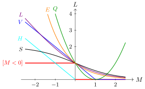
The threshold loss (red) and its continuous approximations as functions of the margin . All of them except pass through the point .
| Loss function | Method | |
|---|---|---|
| threshold | ||
| piecewise linear | support vector machine (SVM) | |
| piecewise linear | Hebb's rule | |
| logarithmic | logistic regression (LR) | |
| quadratic | Fisher's linear discriminant (FLD) | |
| sigmoid | artificial neural networks (ANN) | |
| exponential | the AdaBoost linear ensemble |
You will say that some of these functions are not upper approximations at all: how is an upper approximation? But we can add one to it, and it will be an upper approximation, and that will not affect the solution of the optimization problem. And why a quadratic function that also penalizes overly large positive margins — we will get to that miracle in due course, towards the end of the semester, and see when it happens.
The linear classifier is a model of a neuron
Now let us talk in more detail about binary classification, and specifically about the linear classifier model. It is a model of a neuron, the elementary building block of all modern neural networks, but also a perfectly useful classification model in its own right, which works in many applications. It was invented long ago, in 1943.
A nerve cell is of course much, much more complex than any picture, but this is a model, and a very physical one. A nerve cell has many input processes — dendrites, which can number in the thousands. They let charge into the cell; once inside in a significant amount, exceeding some activation threshold, the charge activates the cell, it becomes excited and transmits an impulse along a long axon to the next cell, where the axon is connected to the dendrites of one or more other cells. So the impulse is passed from cell to cell. What matters for us in this model? Charge, as we know from physics, is an additive quantity: charges add up. Dendrites may let through not all the charge but part of it, and may even inhibit its passage. Hence the linear model: are the charges at the input dendrites; with weights they get inside, form a total charge, which is compared with the activation threshold , and if activation occurs, the function — for example, a threshold one — emits an impulse.
Definition (The McCulloch–Pitts neuron model). The linear neuron model of McCulloch and Pitts [1943]:
where is the activation function (for example, , or ), are the weights of the synaptic connections, and is the activation threshold.
The McCulloch–Pitts neuron model (slide).
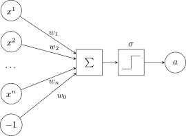
The McCulloch–Pitts neuron: the feature values come in with weights , the threshold acts as the weight of a constant input ; the sum passes through the activation function .
Linear models, first, are what multilayer neural networks are built from, and second, the linear model as a classifier on its own is itself used to solve applied problems.
The stochastic gradient method
We agreed that we use some loss function, and for generality I will write it as . In regression the loss depends on the object , the correct answer and the parameter vector ; in classification, the same. So as not to be distracted by secondary details of whether we are solving regression or classification, let us assume that for each object some loss function is given, smooth — that is important — and depending on the parameters , and we need to minimize the sum of such functions over all the objects of the sample. In each particular problem can be written as a formula; the main thing is that the formula will have to be differentiated.
Definition (The general statement of the learning problem). Given: , the training sample; , , a parametric model.
Find: , the parameter vector of the model.
Criterion — empirical risk minimization:
Gradient descent
For some this is a reminder, for others fresh news — how numerical optimization methods work. I will not go deep into details: we need only the simplest method, the first-order gradient method. Any schoolchild can understand it. Take some point as the initial approximation, and then go in the direction of the fastest decrease of the function. How do we know which direction that is? The gradient — the vector of partial derivatives of the functional being optimized — shows the direction of fastest increase of the function, and we need the steepest decrease, so the antigradient:
Each iteration is a little step of size in the direction of the antigradient. In optimization is called the gradient step, in machine learning the learning rate. If we substitute our functional here, we get a sum of the gradients of the losses over all the objects of the sample:
This is a very important construction for us, and it has a drawback that immediately leads to an idea. We compute the gradient of the loss at the point in a loop over all the objects of the sample: for the first object, for the second, and so on for all, and then add them up and get the next iteration. The question: since we have already computed the gradient step for one term, for the th object, can we not shift at once and update the vector ? Will convergence then not be faster? Another question arises immediately: must we update one object at a time — perhaps collect a whole pack of objects, a batch, and take a step on it? That is possible too, and it is done.
The idea of speeding up convergence is rather old — it is the Robbins–Monro method, invented back in the fifties. If the original criterion is a sum of a large number of terms, then, since taking a gradient is an additive operation, let us take small gradient steps on each term and update the parameter vector more often.
The algorithm
Definition (The stochastic gradient method SG). Input: the sample , the learning rate , the forgetting rate . Output: the weight vector .
- Initialize the weights , .
- Initialize the estimate of the functional on a small random subsample.
- Repeat:
- pick an object from at random;
- compute the loss: ;
- take a gradient step: ;
- estimate the functional: ;
- until the value of and/or the weights converge.
H. Robbins, S. Monro. A stochastic approximation method. 1951.
How to initialize the weights I will put off for now. We need some estimate of the functional already at the zeroth iteration, at least a rough approximation, and there is no point computing it over the whole sample: we are doing everything roughly now, so we take a random subset.
An important point is that the object at each iteration is chosen at random, hence the name: the stochastic gradient method. Why randomness here? It was found that if you keep going through the objects of the sample in a loop in the same order, sometimes the process starts cycling. If the objects are taken in random order, all these artefacts are destroyed and there is no cycling. This is an important discovery, and it is in fact the merit of Robbins and Monro.
We repeat the steps until the process converges. How will we know? The value of has stopped changing significantly, or the weights have stopped changing significantly. In general, in optimization theory the stopping condition is always a heuristic: you can simply set the number of iterations, which is often done in practice, or you can construct very clever combinations of conditions that stop the process earlier, when continuing it no longer makes sense.
Recursive estimation of the functional
Where did the convex combination formula in step 3.4 come from? We want to track how the functional being optimized changes. We saved a great deal by taking only one term, one object, for the gradient step. But the value of is computed over the whole sample, and if we recomputed it over the whole sample each time to track , that would kill all the performance just gained by the stochastic gradient method. We can save by using a recursive formula.
Let us start with the arithmetic mean of the values — at the current step, the previous one, the one before that, and so on. Recursively it is computed very simply — as a convex combination of the previous mean and the last term:
Now replace with . The number of iterations grows at each step, but we use a trick: we fix . The recursive formula for the arithmetic mean turns into a recursive formula for the exponential moving average:
The coefficients decrease into the past as a geometric progression: information about past errors is forgotten at the rate of a geometric progression. The parameter is the forgetting rate of the history of the series. A very useful technique; we will come back to it more than once. Comparing the two recursive formulas shows how to set : it is of the order of , where is the number of values we want to average over. If we want to average over roughly the last ten iterations, ; over a hundred, . In reality the averaging is over all iterations from the very beginning, but roughly speaking one can say it is mainly over the last .
Speeding up convergence: momentum and the accelerated gradient
We will talk about this in more detail in the lecture on neural networks; for now, briefly. If we head for the minimum from some random point, at each stochastic gradient step the object is chosen at random and only one term is optimized. On average we move in the direction in which the total function decreases, but the motion resembles that of a Brownian particle: a random factor keeps pushing us in different directions — bang one way, bang another — though on average we go where we need to.
Can we go where we need to faster? Yes, by averaging the directions each stochastic gradient step gives. The idea is exactly the same as in the exponential moving average — I told you about it just now for a reason; but there we averaged the value of in order to estimate it, and here the motive is quite different.
Definition (Momentum and the accelerated gradient). Momentum — the exponential moving average of the gradient over the last iterations [B. T. Polyak, 1964]:
NAG (Nesterov's accelerated gradient) — stochastic gradient with momentum [Yu. E. Nesterov, 1983]:
If is close to one, we average the gradients over many steps and get a direction that shows more accurately where the criterion decreases. The method was invented by Boris Teodorovich Polyak; it is already considered a classic and a very effective way to speed up the convergence of gradient methods substantially.
The word momentum should be translated into Russian not as «момент» but as «импульс» or «инерция»: it is about the inertia with which the process — a ball — rolls into a potential well, in the direction in which the functional decreases. The oldest gradients we remember with smaller weights, but in fact all gradients from the very first iteration are averaged. Each object adds its gradient vector to the momentum, and this contribution keeps its influence in the vector for a long time. So we move by inertia in the direction set by all the previous objects.
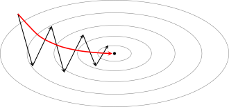
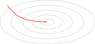
The black arrows are steps along individual stochastic gradients: towards the minimum on average, but with Brownian tossing. The red one is motion with momentum: an averaged direction, corrected at each step, much more stable.
Another interesting way of speeding things up was invented by Nesterov in 1983 — Nesterov's accelerated gradient. We know the direction in which we are moving by inertia, yet for some reason we compute the gradient at the point where we were. Let us compute it at the point we will approximately get to. It turns out that such a small modification — the gradient's argument changed just a little — also leads to acceleration. Together these two techniques can help the iterative process substantially.
Heuristics of the stochastic gradient method
Let us gallop through various heuristics invented to speed up the stochastic gradient method. Some of them are tied closely to linear models, some are more universal.
Weight initialization
How should the weights be initialized at the first step so as to land at a reasonably good point?
- Small random values. Forget this recommendation as a universal one: it comes from old textbooks, nobody does that any more. It is needed only when the loss functions or the activation functions in neural networks have horizontal asymptotes. Then large weight values may knock us into a region where the derivative of the loss is close to zero and the gradient steps come out small. For such problems — yes, random initialization near zero; but that is far from needed everywhere.
- By correlation. An interesting recommendation for linear models:
This is something like the correlation of the vector of values of the th feature on all the objects of the sample with the vector of answers: if a feature is a good predictor for a one-dimensional prediction of , it gets a large weight. There is a justification too: if the features do not correlate with one another and the loss is quadratic, this formula is nothing other than the exact solution of the least squares problem. In practice this almost never happens, the assumption is completely impractical, but as a zeroth approximation — why not.
- Rough training on a small subsample. For example, for a linear classifier the direction vector can be roughly determined like this: take a random object of class and a random object of class , and their difference as vectors in gives the direction from the negative class to the positive one. If we take a few dozen such pairs and average them, we get a much better direction, roughly showing how one class differs from the other. A huge number of heuristics of this sort can be invented.
- Multistart — repeated runs from different random initial approximations, choosing the best solution. Especially appropriate when parallel computing is available: we run the iterative process in parallel from a random set of initial approximations, after some number of iterations choose the best, and can multistart once more from the neighbourhood of that best one.
The order in which objects are presented
Stochastic gradient means that objects are chosen one at a time in random order. Must it be random, and can some non-randomness not be brought in to speed up convergence? Here too there is a huge number of heuristics.
- Shuffling — for example, alternating objects of different classes. The assumption is: if we take an object similar to others that are classified reliably, the gradient step will be small, so it is worth taking objects that differ substantially from each other, and objects of different classes do differ.
- Selecting objects by margin. One can look at the margins introduced at the beginning of the lecture. If the margin is large, the object can be skipped altogether: all is well with it anyway, and gradient steps on it are useless. And if the margin is large in absolute value and negative, things are so bad with it that they will not get better: by taking it into account we will only spoil the classifier. Noise is noise; it would be best ignored altogether. In general: the larger the loss , the higher the probability of choosing .
Around these ideas very many hybrid heuristic methods of speeding up convergence have been invented.
Choosing the gradient step
Another question I have so far swept under the carpet is the gradient step . The theory of optimizing convex functions says that the step should be decreased as the iteration number grows, but neither too fast nor too slowly:
in particular, one can set . One can, but should not, because it works badly; there are theorems about this for convex functions, and if you optimize something more complex, God knows how the step should be decreased. We would like automatic methods for choosing the gradient step.
The method of steepest gradient descent. Take the formula of one iteration of the gradient method and treat the step size as a one-dimensional parameter over which we minimize the loss:
Sometimes this problem can even be solved analytically: differentiate with respect to , set the derivative to zero and find a formula for . But this cannot be done for all loss functions, and then one has to use numerical methods of one-dimensional minimization: the Fibonacci method, bisection, or Newton's method if we can compute the first and second derivatives. The main thing is no fanaticism: there is no need to optimize over super-precisely; it is enough to find roughly for one iteration.
Second-order methods. One can try to improve the first-order method by bringing second derivatives into it. In the first-order method the gradient is multiplied by the step size, while in the Newton–Raphson method it also has to be multiplied on the left by the inverse Hessian — the matrix of second partial derivatives:
The real nightmare here is that the Hessian must not only be computed but also inverted, and it is an matrix, where is the dimension of the parameter vector. Too laborious; nobody does it. How can this formula nevertheless be roughly approximated so as to keep the features of a second-order method, in particular the high rate of convergence?
The diagonal Levenberg–Marquardt method. The Hessian is often diagonally dominant. Let us use a trick: assume that there is nothing in it except the diagonal, that is, the mixed partial derivatives with respect to different variables , are zeros. Of course that is not so, but we simply will not compute them. Inverting a diagonal matrix is a pleasure: it is just ones divided by the second derivatives. But here too not everything is smooth: the second derivatives may be zero or close to zero, they will end up in the denominator, and we will take a random jump due to computational errors. So for stability one more parameter is added to the denominator:
We wanted to get rid of the gradient step parameter, and another one has appeared. But the good news is that the learning rate in the Levenberg–Marquardt method can be set to one: one divided by the second derivative of the loss is in fact an almost optimal gradient step. And is needed where the second derivatives are close to zero — at inflection points, where the loss in the space of is close to linear. Second-order methods do not work there: a second-order method is a parabolic approximation of the criterion being optimized, and it works well where we have almost reached the minimum; that is where the second derivatives give very fast convergence. This is how the gradient step is usually chosen, sometimes by simpler methods, for example by estimating the second derivatives with finite differences; many techniques have been invented.
Advantages and drawbacks of the SG method
So the stochastic gradient method seems wonderful, simple and good, but without additional effort — speeding up convergence, choosing the step, choosing the initial approximation — it may not work very well: converge slowly, get stuck in local extrema, and many other unpleasant things can happen to it. That is why over seventy years it has been surrounded by heuristics.
Its advantages:
- Simplicity: it is relatively easy to implement.
- Universality: it suits any models and any loss functions — as long as the loss can be differentiated with respect to the parameter vector and is smooth. How exactly it is built does not much matter to the method: it is very flexible and can solve a very wide class of problems, not only linear models, both classification and regression.
- Streaming: it can learn from a stream of data.
- Suits big data: it can reach a decent solution having processed only a small part of the training sample, and it often turns out faster and better than more complex and resource-hungry second-order methods.
A few decades ago it was thought in optimization that first-order methods are not very interesting: they converge slowly compared with second-order methods. In machine learning it turned out otherwise. When big data appeared — the functional is a sum over the objects of the sample, and there are millions of objects, sometimes billions — stochastic gradient, especially with momentum, the accelerated gradient and other techniques, turned out to be a real treasure, and one practically does not have to bother with second-order methods. What remains of them is essentially the methods of choosing the gradient step, and real second-order methods can be used only in spaces of small dimension, where the Hessian can be computed and inverted.
The drawback, perhaps, is that one still has to put together a set of heuristics, and that is an art: do not forget overfitting, getting stuck, divergence. True, there are libraries for training neural networks with this very stochastic gradient method inside, and so much invented over the last decades is built into it that we no longer even look inside. We regard it as a reliable engine, a black box that can optimize functions of millions and billions of terms. And this account was so that you have a rough idea of what is under the hood of this black box.
Remark (Escaping local minima and the landscape of the functional). In the lecture someone asked how the problem is solved when the process overshoots a minimum or gets stuck. Among the heuristics there are trial random steps to knock the iterative process out of local minima, but this depends very much on what the landscape of the functional being optimized looks like. Here I recommend Dmitry Vetrov's lectures of recent years: he tells very well how the landscape of neural network functionals is studied now. A lot of interesting things have been found there, and many misconceptions have been run into. It was once thought that this really is a multi-extremal problem and that one has to escape from local extrema by all sorts of methods. Then it turned out that this is not the point: good training comes when a wide minimum forms in the criterion, not just a deep one. A deep and narrow minimum is bad, it is overfitting, it is unstable; a wide and deep one is good. And there turned out to be a huge number of local extrema, all of roughly the same depth, so it does not matter which of them you land in. Such an understanding of landscapes helps set priorities: knocking the process out of local extrema turned out not to be very important, while making the extrema wider is very important, and that is achieved by the choice of neural network architectures.
Multicollinearity and regularization
The stochastic gradient method is surrounded by heuristics, but never mind that. Here, though, is a fundamental problem that shows up in linear models — the problem of multicollinearity; for linear models it is also the problem of overfitting. The point is this: some features may be linearly dependent. In particular, if there are fewer objects than features, there will certainly be linearly dependent features.
What is bad about that? Suppose we have built a binary classifier . Multicollinearity is the condition that there is a vector such that for any object the scalar product : with some coefficients the features can be added up so that the result is always zero. Then the solution is not unique, and therefore unstable. One can always add to : in the scalar product with the addition collapses, , and the classifier will work exactly as the original one.
Definition (Multicollinearity). Multicollinearity is a linear dependence among the features:
Then the solution is not unique: .
The scalar can be anything; it can be sent to plus or minus infinity, and the weights of the features will run off to plus or minus infinity. But the features are collinear only on the training data. Introduce small errors into their measurement, and the addition instantly stops being zero. Then the scalar product flies off to an unpredictable place. Our learning method was looking for the optimum of the functional under multicollinearity and landed at some unknown point of the linear manifold of solutions. The optimum is unstable. This shows up as follows:
- the coefficients go haywire: weights that are too large in absolute value and of different signs appear;
- the discriminant function is unstable: change the vector ever so slightly, and its value flies off who knows where;
- overfitting: . On the training sample the classifier is fitted and everything seems fine, but on an independent control sample everything is bad because of this instability.
Remark (Multicollinearity in practice). In the lecture someone asked: is it right that for an infinite set of solutions it is enough for just two features to be linearly related? Yes, two are enough. And in practice this happens quite often, and not out of malice but when people meant well. Picture a credit analyst who prepares the data for the «grant a loan or not» problem. They have the borrower's income, the income of the borrower's wife, and the family income. But for many people husband plus wife is the family, and for most observations the third feature turns out to be the sum of the first two: there you already have approximate multicollinearity. They wanted to add informative features, but the analyst knew nothing of linear algebra. There are much more hidden situations, when dozens of features depend on each other for a nontrivial reason we do not know in advance: we can build implicit linear dependences into the very measurement or computation of the features, and not only by formulas — they may really exist in nature.
How to fight it? In the course we will see at least three ways:
- regularization: (weight decay);
- feature selection: , ;
- feature transformation: , .
Let us now discuss the simplest. As doctors say, the treatment is symptomatic. If there are infinitely many solutions, a whole manifold, and many of them run off to plus or minus infinity, let us choose among all the solutions the most stable one in the sense of the minimum norm of the vector : minimize the coordinates of in absolute value as far as possible. That is why the technique is called weight decay. The functional leads us into a linear manifold of solutions, and we say: from this manifold we will choose the solution closest to the origin. A second criterion has appeared, the squared norm of the vector , and we add the two criteria with some coefficient .
Definition (Regularization by the norm). Regularization by the norm (weight decay) is a penalty on increasing the norm of the weight vector:
where is the regularization coefficient.
This technique is also called stabilization, but most often regularization. It is completely standard, and for linear models simply obligatory, because we do not know whether there will be overfitting due to multicollinearity. Let us see what happens to the gradient vector: a small correction has been added to it — because it is a squared norm, and with at that:
The modification of the gradient step in the SG method is, one could say, an edit to one line of code:
We simply multiply the vector from the current iteration by a number less than one — there it is, decay, shrinking, reducing the norm of the vector — and take the gradient step in the same direction as before. A very simple implementation.
Remark (When regularization is appropriate). This technique is called regularization because here is the norm of the vector . In the next lectures I will show completely different techniques for overcoming multicollinearity. Another important point: multicollinearity in this form is characteristic only of linear models. In showing that instability arises, we relied essentially on the linearity of the model. If the model is nonlinear, doing regularization is, generally speaking, rather silly. One has to look: perhaps a weighted sum of features is still sitting somewhere inside, and then regularization is useful. But sometimes models are built quite differently, the features enter the formulas in another way, and there it is not needed and will not work. Whether one regularization or another is appropriate follows from our having understood the nature of the instability of the solution. Here that nature is linear dependences among the features.
The probabilistic statement of the classification problem
Another fundamentally important paradigm in machine learning, and an important message of today's lecture, is the probabilistic statement of the problem. Suppose the Cartesian product is a probability space with some density, and the «object — answer» pairs, both from the training sample and from the control one, are generated by this joint distribution independently: i.i.d. (independent identically distributed). In mathematical statistics such samples are called simple. Our task is to estimate the joint density from the sample: if we have an estimate of it, we will be able to compute the probability of the class for any object .
What does it mean to find the density ? We solve optimization problems over parameters all the time, so parameters must be introduced into the density. The density factorizes by the formula of conditional probability, which is always true, and we introduce the parameter into the model of the conditional probability of the class — that is convenient for us. The alternative approach, where the parametrization goes the other way round, we will also consider later. How to specify the model itself we will put off for now; first let us deal with the optimization criterion.
Definition (The maximum likelihood principle). Let be a probability space with density , and a simple (i.i.d.) sample from . The problem is to estimate the density from the sample . The parametric density model:
where is the conditional probability of the class with parameter , and is an unknown, non-parametrizable distribution on .
Maximum likelihood (Maximum Likelihood Estimate, MLE):
Maximum log-likelihood (log-likelihood, log-loss):
The maximum likelihood method is one of the fundamental methods of mathematical statistics and machine learning, and we will use it far and wide as soon as we talk about a probabilistic model of data generation. Once upon a time there was a density, objects were generated from it, and now we observe them. The direct problem is to generate objects from the density; we have to solve the inverse one: from the observed objects say what density could have generated them.
The likelihood of the data is the density of the whole sample with our data substituted into it. Why is it a product of densities over the individual objects? Because we assumed independent generation: the density of an independently generated sample equals the product of the densities of the individual pairs. We substitute the factorization of the density, and we are entitled to drop the factor : it does not depend on . We need the density in order to say for which from the parametric family the generated sample is most likely. This is the maximum likelihood principle: choose the parameter of the generating density for which the observed data is most likely.
A product over all the objects of the sample is inconvenient for optimization, so one takes its logarithm: the maximum point of a functional and of its logarithm is the same. This is a completely general technique. As soon as you read about a probabilistic model of data generation, expect optimization of the log-likelihood two lines later. We get a sum over all the objects of the sample, and the logarithm of the model of the conditional class probability is nothing other than a loss function — more precisely, minus the logarithm: here we maximize, while losses are usually minimized.
Remark (If the observations are dependent). Someone asked: if the independence assumption is wrong, what methods are used? A very good question. What does «wrong» mean? Can we model the dependence? If we can, there is a whole package of different methods. For example, if an object depends only on the previous one, the objects form a sequence: a time series, a Markov process, Markov chains. The dependence assumption enters the model explicitly there, and there are techniques of its own, like maximizing likelihood, only the theory is different. There are many such theories, but let us deal with the classics first. Practically our whole course, except literally a few lectures, will be about independent observations: it is the most textbook and most frequent situation. Mutual dependences in data — deep neural networks, for example — will come next semester.
Likelihood and the approximated empirical risk
There is a close link between maximizing likelihood and minimizing empirical risk — I have in fact already let it slip. Let us look at the same classification problem in two ways. On the one hand, we can build a probabilistic model of classification, for simplicity with two classes. On the other hand, we can say: we have no probabilistic hypothesis, no probabilistic nature of the data. We build a separating surface between the classes, we take a purely geometric view of the problem, and as the model we fix a parametric family of discriminant functions. Let us write out the two criteria that arise in these two paradigms.
Maximizing likelihood, where is the model of the conditional probability of the class :
Minimizing the approximated empirical risk, where is the model of the separating surface, :
Both are sums over all the objects of the sample, where some loss is written for each object, and it is tempting to say that they are the same thing. Each term depends on only one object, so they can be equated independently.
Proposition. These two principles are equivalent if we set
The model the model and the loss function .
Then the probabilistic approach is merely the construction of a separating surface with such a loss function. A dual view appears. People of different faiths may come: some believe in probability and that the world around us is probabilistic, while others regard probability as a strange thing — where in life have you seen algebras of measurable events? — and use pure geometry. Both are right, and they can be reconciled. You do not believe in probabilities, you have written out a separating surface and a loss function ? Look at this equality: I will take its exponential and say that this is the probabilistic model of the data. And from the other side a probabilist comes and says: «I am modelling the data». And we tell them: «Nothing of the kind, you are building a separating surface with such and such a loss function». These are two legitimate, equal, dual views of what we are doing. Whether to use the probabilistic paradigm or not is a matter of taste, a matter of which model of the world we believe in.
Remark (Notation). Watch the notation: a small is always a probability density with me, in general of a continuous distribution, and a capital is always a discrete probability, for example the probability of a class. There is a finite set of classes, and if we sum over all , we get one — the normalization.
The probabilistic meaning of regularization
Since with this transition we can freely jump between the probabilistic and non-probabilistic paradigms, let us ask: what, in probabilistic language, is the regularization that arose for linear models?
Suppose there is a probabilistic data model . Who is , where does it come from? Until now was a non-random parameter that we found from the sample by maximum likelihood. Now suppose that is also a random vector, generated from its own distribution. This is a two-level model of data generation. The space is, as it were, the space of the practical problems we face. The Lord God generates a problem from a prior distribution and slips it to us, and then a training sample is generated from this problem; we look at the data and try to determine the model. If we know the model of problem generation the Lord God uses, we can bring something extra into the solution.
Definition (The maximum a posteriori principle). Let be a probabilistic data model; the prior distribution of the model parameters; the vector of hyperparameters. Now not only the appearance of the sample but also the appearance of the model is taken to be stochastic.
The joint likelihood of the data and the model:
The maximum a posteriori principle (Maximum a Posteriori Probability, MAP):
The hyperparameters are again a non-random vector, parameters over parameters. Since the likelihood has been formalized this way, nothing prevents us from writing out the maximum likelihood principle, which in this case is called the maximum a posteriori principle; it too is used very often in probabilistic statements of machine learning. The logarithm of the joint density gives two terms. The first is our old acquaintance, the probabilistic loss (if taken with a minus). The second, the logarithm of the prior distribution, does not depend on the data; it is a criterion on the parameters. That is, it is a regularizer.
Again two paradigms. In one we say: we have peeked into the heavenly chancellery and know from which distribution problems are slipped to us for practical solution. In the other, we are solving an ill-posed problem and have therefore added a reasonable restraint, a regularizer. These are two equivalent languages, and which of them to formalize the problem statement in is a matter of taste.
Remark (Probabilistic methods and small samples). Someone asked whether probabilistic methods work on smaller samples. I am trying to show precisely that the two approaches are equivalent, and the problem is expressed in that very regularization. A small sample makes the solution unstable: the functional being optimized lacks terms, there are too many parameters, and too little data to determine them. That is the essence of the trouble called «small data». If there is little data, we will certainly have to make some prior assumptions about what the parameter vector looks like. There you have regularization — probabilistic if you like, or some other kind, and in what language you formulate it does not matter.
The Gaussian and Laplace priors
Since we have agreed that prior distributions, or rather their logarithms, can play the role of regularizers, let us make these assumptions: the weights are independent, the expectation of each is zero, and the variance is some constant :
Example (The Gaussian distribution and the quadratic () regularizer).
We take the logarithm and — an astonishing thing — get our acquaintance, the regularizer of the linear model. On the other hand, in probabilistic language we say that the parameter vector is somewhere in the neighbourhood of zero and does not run too far from it: there it is, a probabilistic assumption, a constraint on the variance. The regularization coefficient turns out to be inverse to the variance: the larger the variance, the weaker the regularization, and vice versa. A small variance means we press the weights hard towards zero, so the regularization coefficient is large.
Example (The Laplace distribution and the absolute () regularizer).
is a hyperparameter, is the regularization coefficient.
The Laplace distribution resembles the Gaussian, but instead of the square it has the absolute norm — the sum of absolute values. This is a very interesting regularizer. regularization, weight decay, shrinks the coefficients: they decrease but do not reach zero. With regularization the effect of zeroing coefficients arises: the corresponding feature is simply not used; the regularizer switches features off. We will have many occasions to talk about this in the course.
We will discuss logistic regression and the example of the credit scoring problem another time.
Remark (Regularization and Bayesian methods). After the lecture someone asked: they say the number of parameters has caught up with the amount of data, and under such conditions maximum likelihood starts to fail, so Bayesian methods now have priority? Not quite. Regularization has priority: the concept of regularization is more important in principle, and the Bayesian method is a special case of it. Bayesian regularization is when, as in this lecture, the constraint is specified as a prior distribution of the model parameters. But regularization can also be done not in probabilistic language. It has a huge number of techniques: additional terms in the criterion being optimized — sometimes they can be interpreted as the logarithm of a prior distribution, and then it is Bayesian regularization, and sometimes they cannot; heuristics inserted into algorithms; in deep neural networks, something unusual in the architecture.
It is precisely such findings that made it possible to build huge models from a comparable amount of data: language models and computer vision models of fantastic depth, with hundreds of layers, billions of parameters and billions of training examples. Overfitting should have been simply wild, yet it is not — because several techniques are used inside. One of them, dropout, which I will talk about when we get to neural networks, does not look like regularization at all. Another was invented first in convolutional networks for computer vision — the skip connection. Its essence is that a whole layer of the network starts working as a small correction to the previous layers; it has nowhere to go, it must be small. This too can be interpreted as regularization, but not always conveniently — specifically as a Bayesian prior. Though that, of course, is a matter of taste, or even of faith. If a scientist works on some approach for years and puts their soul into it, they will generalize it and extend it to situations where it seemed not to work before. This is a very justified direction of research, and after a number of successful works one can come to the conclusion that everything in the world is Bayesian learning. It can be interpreted that way too, but it is not obligatory: it is the researcher's individual choice.
No comments yet
Be the first to share your thoughts.