August 30, 2026 · Lecture · LibreTimes
Machine Learning 1. Lecture 1. Basic Concepts and Examples of Applied Problems
Contents
- What this lecture is about
- The problem of learning from examples
- How objects are described: features
- How answers are given: types of problems
- Fisher's irises
- How models are defined
- Feature generation
- Training and application
- Loss functions and empirical risk minimization
- The Runge example
- Underfitting and overfitting
- Empirical estimates of generalization ability
- Examples of applied problems
- Medical diagnosis
- Recognizing mineral deposits
- Credit scoring
- Predicting customer churn
- Text categorization
- Biometric identification
- Predicting real estate prices
- Forecasting sales volumes
- Complexly structured data and deep learning
- Peculiarities of the data and of the statements of applied problems
- The CRISP-DM standard and the evolution of artificial intelligence
- Experiments in machine learning
- Summary
- Seminar
What this lecture is about
This is an introductory lecture in two parts. The first part gives the definitions and notation we will use throughout the course. The second is a quick run through examples of applied problems: what objects, features and answers can be, and what specifics arise in each problem that have to be taken into account at the modelling stage.
Everyone is talking now about deep neural networks and artificial intelligence, and we will deal with such things too, but in the second semester. The first semester covers the more classical machine learning problems, those that involve processing matrix data. The course is theoretical: practice is in other courses and in the seminars.
The problem of learning from examples
In machine learning we solve non-standard problems of function approximation — roughly speaking, we draw a function through given points. We are given a set of objects and a set of answers, and we assume the answers depend on the objects somehow: there is an unknown target dependence, and it has to be recovered from empirical data. On a finite set of objects the answers are known — this is the training sample — and we need to find a function that gives an answer for an object.
We will denote this function by the letter , for «algorithm»: it matters a great deal to us that it can be computed on a computer. So I will often say «algorithm», and sometimes just «function».
Definition (The problem of learning from examples). is the space of objects; is the set of answers (predictions, estimates, forecasts); is the unknown dependence (target function).
Given: , the training sample, on which the answers are known; , a parametric model of the dependence.
Find: a parameter vector such that .
Criterion — the minimum of empirical risk:
(empirical risk minimization, ERM), where is the loss function: the more deviates from the correct answer , the larger it is.
The whole course will answer four questions: how objects are described, what the answers can be, in what sense approximates — a nontrivial question — and, finally, how to build the function . The last question is the constructive part of the whole course.
How objects are described: features
Objects are described by features. In Russian everyone now says «фичи», a borrowing of the English word, but I do not like it: for half a century Russian has said «признаки», and mathematical statistics says «факторы». That is the established Russian terminology, so let us use it.
Take credit scoring as an example. A person comes to a bank to ask for a loan; for the bank this person is an object for which an answer is needed: grant the loan or not. There is some information about the person: partly the answers to the questions of an application form, partly formal information from various databases, and some things are checked by the bank's security service. In any case we take measurements of the person, and the result of each measurement is a feature. What matters is that formally a feature is a function of the object, a map from to the set of its admissible values.
Definition (Feature, feature description). The features of objects are functions , . By the set of values the types of features are distinguished:
- — a binary feature;
- — a nominal feature;
- and is ordered — an ordinal feature;
- — a quantitative feature.
The vector is called the feature description of the object .
A binary feature is a «yes» or «no» answer. A nominal one takes finitely many values: for example, the borrower's profession or place of residence. An ordinal one is, for example, education: primary, secondary, higher, an academic degree; here one sees that the values are ordered. The order need not be total: it all depends on the situation; sometimes ordinal features are linearly ordered, sometimes the order is only partial. A quantitative feature is the most frequent case, when we measure something about the object in numbers.
We have numbered all the ways of measuring an object and always use them in the same order, so the feature description is a vector. If we measure all the features on a finite set of objects, we get the «objects–features» matrix (feature data):
Rows correspond to objects, columns to features, and inside are the measurements of each feature on each object. Not every feature is measured on every object, so this matrix has missing values: a matrix with holes is a perfectly ordinary situation.
How answers are given: types of problems
The answer is also a function of the object, the target function that we recover, and we look for a function that approximates it. Depending on the set in which both functions take their values, problems fall into large classes.
Classification problems: is a finite set. Usually this is a decision from a discrete set of options: grant a loan or not, what diagnosis to give a patient, what treatment to prescribe.
- or — classification into two classes (binary classification);
- — into disjoint classes (multiclass classification);
- — into overlapping classes (multilabel classification).
The most basic is classification into disjoint classes, when an object can belong to only one class, though there may be many classes. For example, in optical character recognition each position holds one particular letter, and it has to be assigned one of the classes. But in medical diagnosis a person may have a whole bouquet of diseases — a stomach ulcer, and epilepsy, and something else. That is a problem with overlapping classes, and the models for these two situations are built differently.
Regression problems: or . For an object we need to predict a numerical answer — any number from minus to plus infinity. Why the problem has such a strange name, we will discuss when we get to it.
Ranking problems (learning to rank): is a finite ordered set. The objects have to be put in order. This problem sits between classification and regression: on the one hand, an object must be assigned an integer rank; on the other, the methods used are closer to regression: to order objects, one builds a model that outputs some quantity on them, a score, and ranks the objects by it. A separate lecture in the second semester will be devoted to ranking methods.
All of the above is supervised learning: the correct answers are given on the objects of the training sample. There is also a large class of unsupervised learning problems, where there are no answers at all and something has to be done with the objects themselves. We will reach those only at the end of the semester.
So supervised learning is learning from examples, recovering dependences from empirical data, predictive modelling, approximating functions through given points: all these are synonyms. The two main types of problems are classification and regression, and it helps to keep two pictures always before your eyes.
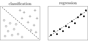
On the left, classification: we need to build a separating surface between two sets, the circles and the crosses. On the right, regression: we need the dependence of (on the vertical axis) on (on the horizontal one). If you can picture these two images, that is already enough as a basis for thinking about the problem.
Fisher's irises
A textbook example — soon it will be a hundred years old. Ronald Fisher, who did a great deal in mathematical statistics, collected a training sample of 150 iris flowers back in the pre-computer era: three species of the plant, 50 specimens of each, and for each flower he measured four features — the length and width of the sepal and the length and width of the petal.
What is good about this problem? First, it is very simple. Second, if you plot the features pairwise — sixteen pictures, each feature against each — you can see that the clouds of points of each class are in effect probability distributions. That is what led Fisher to the idea of describing classes in classification problems by probability distributions; we will get there when we talk about Bayesian classification theory towards the end of the semester.
The value of such a visualization is that it shows at once whether a problem is easy or hard. Already in one of the pictures you can see that Iris setosa separates very reliably, while the other two species overlap somewhere — and ideas immediately come about which mathematical methods could separate them. On the plane we see the projection of the sample onto two particular features; it is hard to visualize in the axes of all four, but apparently in four dimensions it separates even better than in two. Such visualizations, where features are plotted against each other pairwise, are very useful in practice.
How models are defined
Once we have talked about the data and understood that objects are described by feature vectors and we want to predict , it is time to decide what exactly we are building.
Definition (Model). A model (predictive model) is a parametric family of functions
where is a fixed function and is the set of admissible values of the parameter .
The function is fixed: it is simply a formula we can write down. It depends on the features and on unknown parameters, and it is these parameters that we will train.
Example (The linear model). The linear model with the parameter vector : multiply each feature by a weight that is unknown for now and add everything up:
— for regression and ranking, ;
— for classification, .
Can always be predicted by a linear combination of features? Probably not: not every model in the world is linear. But sometimes it can. What makes up the price of a flat? Its floor area, the number of rooms, whether it has a balcony, the distance to the metro, and so on. Each feature contributes to the price, and to a first approximation the contribution can be considered linear.
In a classification problem we are interested not in the value of the linear combination itself, this score, but in the decision. So we wrap the linear combination in the sign function: if it is greater than zero, the object goes to class ; if less, to class . We will study linear models both for regression and for classification.
Feature generation
Here is an example where there are three features, though the problem was one-dimensional to begin with: we need to predict from . The points are pairs , , , and a function has to be drawn through these points.
Here we use a trick, and it is a conceptually very important technique that often proves useful in practice. Formally a feature is a function of the object. Our object has a single measurement , but as a feature we can take any function of it: , , , — and so multiply one feature into many new ones by functional transformations. Take the three features and build a linear model on them; or take the features and build another:
After fitting the parameters one sees that these two models approximate the data differently: in this case the model with the sine did slightly better than the parabolic one. Two conclusions follow:
- computing new features can enrich a model;
- in practice it is very important to guess the model, to find as adequate a one as possible.
Training and application
We are beginning to see that we solve any supervised machine learning problem in two stages.
Definition (Learning method). A learning method (learning algorithm) is a map
that builds the function from the training sample by estimating (optimizing) the model parameters .
At the training stage (train) we have a training sample — objects and the correct answers on them — and from it we build an algorithm that will give an answer for an object:
This is the most important and the hardest stage in solving machine learning problems.
At the application stage (test) the function we built gives answers on new objects :
Say we had historical data on thousands of borrowers about whom it is already known whether they repaid their loans, and from it we built a credit scoring model. Now a new person comes in; we know nothing about them yet, but the model says: this is a good borrower, their probability of default is 1%, and the loan can be granted. The application stage is usually very simple: a function already built has to be applied to a new object.
Remark (Notation used throughout). Throughout the course I will try to keep the same notation: for objects, for answers, for the index of a feature, for the index of an object, for the length of the training sample. It is worth remembering, so as not to spend time loading the notation into memory and working out what is what.
Loss functions and empirical risk minimization
How is the learning problem solved? Machine learning is always optimization. This is one of the most important messages of today's lecture, and of the whole course: reducing the problem of approximating a function, the learning problem, to an optimization problem is the first step you must be able to take in any state. Wake you up in the middle of the night, tell you a machine learning problem has to be solved urgently — first of all you write out the sum over all the objects of the sample, then the loss function, and only then do you switch on your brain and start thinking.
The loss function characterizes the algorithm's error on an object.
For classification problems the answers and are elements of the same discrete set, so the natural loss function is simply the error indicator:
Remark (Iverson notation). The square brackets are the so-called Iverson notation; Donald Knuth used it very widely and popularized it in his books. The square bracket turns «true» into one and «false» into zero, that is, a logical expression into an arithmetic one. It is very convenient in writing, and from now on I will use it without further reminders.
For regression problems, the absolute difference or the squared difference:
Next we write out the criterion we will optimize: the empirical risk, or the quality functional of the algorithm on the training sample — the sum of the losses over all the objects of the sample:
Practically all machine learning problems optimize exactly such functionals — sums over all the objects of the sample. This is very convenient; many methods explicitly use the fact that it is a sum, and we will soon meet them: neural networks, for example, are also trained only on functionals with a sum in them. The convenience is purely mathematical, but so strong that we do nothing else.
Remark (Sum or mean). Sometimes the arithmetic mean is taken instead of the sum. From the optimization point of view there is no difference: the functional can be multiplied by any positive number, any number can be added to it, and moreover any monotonically increasing function can be applied to it, and the minimum point will not change. Where a sum is more convenient and where a mean — it makes no difference to the statement of the problem.
Definition (Empirical risk minimization). The method of empirical risk minimization picks from the model the algorithm that minimizes the empirical risk:
This is one of the main general problem statements in machine learning. Get used to this notation: a small from the parametric family capital that minimizes the criterion written out.
Example (The method of least squares). A regression problem, numerical features, a linear regression model — all features with some weights:
and the quadratic loss function. This gives the method of least squares, a special case of empirical risk minimization:
If the loss function were different, it would still be empirical risk minimization, just with a different loss function. The general statement is empirical risk minimization; the special one is least squares; and if a particular model is also given, a linear combination of features with coefficients, then it is already a concrete mathematical problem for which there is a heap of concrete methods, and we will study them too.
A problem can be solved when it is well posed — when it has its DNA, which in Russian reads as the initials of Дано (given), Найти (find) and Критерий (criterion). Here what is given is the training sample; what is to be found is the model parameters, in this case of a linear regression model; the criterion is the least squares criterion. It is more precise to say «criterion» or «least squares functional», and to call a method the numerical algorithm that will solve this optimization problem. There are many such methods.
The Runge example
Take a particular function that even has a personal name — the Runge function. Runge once came up with this example to show that polynomials are not a very good way to approximate functions with horizontal asymptotes. The function looks like a little hat:
The feature description of an object is — all powers of from the zeroth to the th; the polynomial regression model
is a polynomial of degree ; training is by least squares:
The training sample is the values of the function at the nodes of a uniform grid on the interval, the control sample is the values at the nodes of the same grid shifted by half a step, that is, at the points midway between the training ones:
The control sample is needed to see not only how well we approximated the function at the training points, but also how this approximation works in the gaps between them. The question: what happens to and as grows?
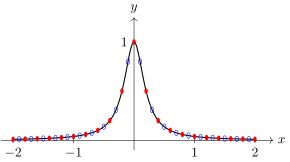
The Runge function on the interval ; in red, the training sample at the nodes of a uniform grid (); in blue, the control sample, at the midpoints between them.
In the lecture I showed what this looks like as the degree of the polynomial is gradually increased. The function is even, so only even powers are needed in the polynomial. With three coefficients — for the square, the linear term and the constant — it is just a parabola; with five, a little better. After that the approximation seems to get better and better, but then a strange wobble begins at the ends of the interval. Note that this wobble concerns only the control sample. The curve passes nicely through the red, training points, and simply horribly through the blue, control ones: inside the intervals between the training points everything becomes very bad. This is exactly what Runge wanted to show.
If the degree is increased further, everything falls apart completely. Here the complexity of the polynomial already plays a negative role: overfitting has begun — we fit the function better and better to particular data, the training sample, while at other points things get worse and worse, and on control material this is no longer any approximation at all. Add to this the accumulation of computational errors: a polynomial of a degree approaching fifty has to be computed carefully. But that is the subject of numerical mathematics, not of our course.
Let us plot the value of the criterion as a function of the degree of the polynomial. When the polynomial is evaluated at the points of the training sample itself, it gets better and better as the degree grows, and it seems to us that we have approximated the dependence very well. But that is not so: on the control sample, from some point on, the error starts to grow.
The Runge example: against the polynomial degree (slide). In red, the training error; in blue, the control error; the triangle marks the optimal complexity.
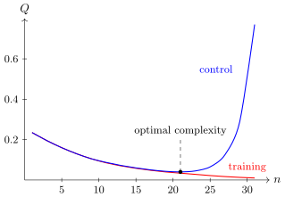
against the polynomial degree (): in red, the training error ; in blue, the control error . On training the error falls monotonically as the degree grows; on control it rises sharply after the optimal complexity.
Definition (Overfitting). Overfitting is when the error of the trained algorithm on the control sample substantially exceeds its error on the training sample:
Remark (The sensitivity of polynomial models). In the lecture someone asked: with a large spread of degrees the model is very differently sensitive to different parameters — is overfitting due only to the number of parameters, or to the nature of the model itself? To both. This example is precisely about a model poorly chosen for the problem: a polynomial model is ill suited to approximating functions with horizontal asymptotes, and the higher the degree, the faster both the computational errors and the error due to overfitting accumulate. When the model fits the dependence poorly and has more and more parameters, those parameters overfit: the function passed nicely through the sample, but the law of nature has not been recovered. Overfitting may come from the complexity of the model, or from the model being taken from the wrong parametric family, not even close to the one containing the unknown target dependence. Then the model has to be changed, a more suitable formula invented. Nobody uses polynomials, especially for such functions. And yes, polynomial models with many parameters are very sensitive to errors in the data: you saw how, at a degree approaching the number of points, the function starts to break even on the stretch near zero where everything seemed fine. These are the accumulated errors — very small ones, due to the finite word length, but when numbers are raised to the fiftieth power they accumulate into something visible to the eye.
Underfitting and overfitting
People observed dependences of this kind from the fifties and even earlier, when such problems were solved before computers. The conclusion was: excessive model complexity is an evil to be fought, it leads to overfitting. From the sixties to the nineties a great many mathematical theories were created about how complexity affects overfitting and why it causes it. Later this was revised. In the mid-nineties boosting appeared — we will talk about it too — which showed that even complex models can be trained very carefully, so that they do not overfit. Then came a heap of techniques for training very complex models, multilayer and deep neural networks. Today we know many ways to fight overfitting, but the problem never leaves us: there has never been a machine learning problem with no overfitting at all. We can aim to minimize it, and we will study many ways of doing so in the course.
Underfitting and overfitting (slide): a model that is too simple, one that fits, and one that is too complex.
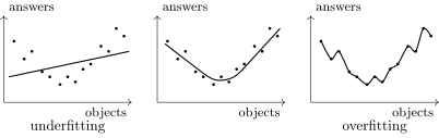
On the left, underfitting: the model is too simple, inflexible. In the middle, a model that captures the dependence. On the right, overfitting: a model with an excessive number of parameters passes through every point of the sample but does not recover the dependence.
These are two extremes, and in every problem we have to steer between Scylla and Charybdis. Underfitting comes from an oversimplified model: we wanted to solve a complex problem and took too simple a model for it — plenty of data, too few parameters, an inflexible model. Overfitting: the model is taken excessively complex — many parameters, too little data — and the excess parameters adjusted themselves to the data but did not capture the dependence. And we do machine learning, after all, in order to learn a law of nature from empirical data.
Where does overfitting come from? We make a decision under incomplete information. We want to build an approximation of the target function, and the target function is known to us only at finitely many points; and we want to decide which model is best — a decision that is inevitably associated with some error. How to minimize this error is another matter; but it can be detected in the way I have already shown in the plots: we always split the sample into training and control, train and test. Train to build the model, test to examine it, and to examine it honestly: here is new data, make predictions. We know the correct answers but do not show them to the model: we are the examiner, we compare its predictions with the correct answers. No practical problem is solved without such a comparison: the data always has to be split into training and control.
Remark (Overfitting occurs even when choosing between two algorithms). I worked on this subject when writing my doctoral dissertation — I defended it in 2010. One of the problems there was simplified to the limit: instead of a parametric family there are just two algorithms, and from a finite sample one has to say which of them is better. Of course, you look at their predictions on the training sample and pick the one whose predictions are better — and with some probability you will be wrong. This probability can be computed exactly and one can study what it depends on: on how different the algorithms are and how good they are. The conclusion: even when choosing between just two or a few options, the probability of overfitting is nonzero. How to make it small is another matter; we will deal with that too, building on the techniques accumulated over seventy years of machine learning.
Empirical estimates of generalization ability
A few words about frequently used estimates based on splitting the sample into training and control.
-
Hold-out is the simplest: split the sample into training and control once:
What is bad about it? The quality will depend on the particular split: we bring some subjectivity into measuring the quality of the model.
-
Leave-one-out, : each object in turn is made the control one. We train times on a sample lacking one object and check how the model works on that very object:
This is an important technique, and we will often use it.
-
Cross-validation, : why make only one object the control one? Let us split the full sample in different ways into a training subsample of length and a control one of length , and average over the splits:
where is the set of splits . There are many variants of splitting and averaging, and we will have a chance to discuss them in more detail.
This completes the first part of the lecture. The main things in it are the training sample, the loss function, empirical risk minimization, overfitting, and the notation we will keep to from now on.
Examples of applied problems
Now a quick run through applied problems — literally a few minutes per problem — to illustrate what features and answers there are and what specifics arise in each problem.
Medical diagnosis
The object is a patient, and an important subtlety: a patient at a particular moment in time. The same person before and after an operation is two different objects for us, or this must be accounted for in the features. What is predicted is, for example, the long-term outcome of surgical treatment; or a treatment method is prescribed; or a diagnosis is made. The classes are a diagnosis, a treatment method or the outcome of the disease: it is a classification problem, a discrete decision problem.
The features are, as a rule, of different types:
- binary: sex, headache, weakness, nausea, etc.;
- ordinal: severity of the condition, jaundice, etc.;
- quantitative: age, pulse, blood pressure, haemoglobin level, drug dose, etc.
A peculiarity is that the data usually has many gaps. Many things can be measured in a person, but each time only what may have at least an indirect bearing on the disease in question is measured, so the data is always incomplete. Besides, as in credit scoring, where the object is also a person, one needs not only to make a decision but also to estimate the probability of an adverse outcome: how to plan the medical measures depends on it.
Overfitting is also clearly visible in this problem. Take the problem of predicting the long-term outcome of surgical treatment of atherosclerosis and plot various decision rules: the error rate on training along the horizontal axis, on control along the vertical. The points are systematically shifted upward relative to the diagonal. Some of them happened to land below it: with some probability control is better than training, but that is pure chance, due to variance. The systematic upward shift means that on training it always seems to us that the model works better than it actually will — sometimes much better. Here is a rule with 4% errors on training: what joy, a good model. And on control it has 8% errors. How large this disaster is, is a very subtle and nontrivial question, solved differently in each problem, but at least we always have a way to measure it: split the sample into training and control and examine the model.
Recognizing mineral deposits
The object is a geological area (an ore field); the classes are whether a mineral is present or not. Features:
- binary: the presence of large zones of crumpling and schistosity, etc.;
- ordinal: mineral diversity, experts' opinions on the presence of the mineral, etc.;
- quantitative: antimony content, the presence of antimonite in the ores, etc.
Our teacher, Academician Yuri Ivanovich Zhuravlev, worked on such problems back in the sixties. It was, as people said then, a task set by the party and the government: to find gold deposits of the South African type on the territory of the Soviet Union. Using mathematical methods that were only just appearing in those years, together with geologists — they were the ones who posed the problem, and all the features and all the data came from them — he found two deposits. History repeats itself: recently a mining company came to me with the problem of searching for diamonds, kimberlite pipes. Decades pass, and the problem does not grow old. Its peculiarity is the problem of «small data»: for rare types of deposits there are far fewer objects than features.
Credit scoring
The object is an application for a bank loan, information about a potential borrower. The classes are bad or good; this is the terminology established among credit analysts. The features are of different types:
- binary: sex, having a telephone, etc.;
- nominal: place of residence, profession, employer, etc.;
- ordinal: education, position, etc.;
- quantitative: age, salary, length of service, family income, loan amount, etc.
In medicine and in lending alike the object is a person, though the information about them is very different. A common subtlety is that one needs not only to decide «good» or «bad» but also to estimate the probability of default : depending on it, the bank's loan portfolio is reassembled in different ways. When we talk about logistic regression, which is often used in banks, we will say a bit more about how the probability of default is estimated. This is no longer quite classification: classification is discrete, while a probability is a continuous quantity from zero to one. So logistic regression, though it solves a classification problem, is in some sense a regression: it outputs a continuous-valued quantity.
Predicting customer churn
Another problem from business. The object is a subscriber at a particular moment in time: for example, a mobile subscriber or a regular customer of a retail chain. The classes are whether they will leave next month or not. There are very many such problems now: a customer has to be kept from going to competitors, preferably in advance. So indirect features are needed for early prediction of a possible departure. These have to be cunning features: for example, the customer's traffic has somehow changed — they changed jobs, their company's corporate standard is another operator, and they were with us. How do we keep them?
Features:
- binary: corporate customer, activated services, etc.;
- nominal: tariff plan, region of residence, etc.;
- quantitative: call durations (incoming, outgoing), SMS, etc., payment frequency, etc.
Peculiarities of the problem: the probability of leaving has to be estimated; the samples are extremely large; features have to be computed from «raw» data. They have to be invented — at least that is how the problem was solved ten to fifteen years ago. With the arrival of neural networks that can process complexly structured data, automatic feature generation is used more and more: we used to sit down as experts and think about which features to invent here, and now more and more often the raw source data can be fed into a neural network model, and it will compute the features itself — we do not even know which, but such that they are as informative as possible.
Text categorization
The object is a text document; the classes are the headings of a hierarchical subject catalogue. For example, incoming messages have to be distributed among the departments that handle requests: thousands of applications and complaints come in from customers, we have thirty departments that solve different problems, and the customer has to be automatically redirected to the people who will help solve their problem. Or the categorization of scientific papers, patents, news items and so on.
The features of a text can of course be word frequencies — in the text, in the headings, in the abstract — as well as various meta-features, that is, information about the document itself: author, publication, year, date and time, the source it came from. Categorization is also classification, and often classification with overlapping classes: one document can be assigned to several headings. Besides, only a small share of the documents have answers .
Biometric identification
Another classification problem, where the number of classes can be very large. A person is identified by fingerprints, by the iris of the eye. The iris is known to distinguish all the people living on Earth: each person's is so individual that there are algorithms that tell them apart with almost one hundred percent reliability. Here is a classification problem with billions of classes — and it is quite solvable. Peculiarities: nontrivial preprocessing to extract features and the highest accuracy requirements.
Predicting real estate prices
Now from classification to regression. The object is a flat in Moscow. The features are again of different types:
- binary: a balcony, a lift, a rubbish chute, security, etc.;
- nominal: the city district, the type of building (brick, panel, block, monolithic), etc.;
- quantitative: the number of rooms, living area, distance to the centre, to the metro, the age of the building, etc.
This problem is interesting because linear models may well work here, but some features have to be transformed. How does the distance to the metro enter the price of a flat? Clearly a monotonically decreasing transformation is needed: the farther from the metro, the smaller the contribution. But how this decreasing function is shaped — whether it resembles a hyperbola of some power or something else — calls for an auxiliary one-dimensional transformation of the feature, so that it can then be included in the linear model. Besides, the sample is inhomogeneous: prices change over time.
Forecasting sales volumes
I worked on this problem myself quite actively about fifteen years ago; a whole startup later grew out of that work, and it is now a successful Skolkovo company. The problem is to forecast sales volumes in a supermarket chain. Here it is not trivial to understand what an object is. In medical problems an object is a person at a moment in time; in the churn problem, also a person at a particular moment in time. Here the object is a triple : we need to forecast how much of the given product will be sold in the given store from the given day over some following period — a week, a month, or, for perishable goods such as meat, a day. The features are binary (a day off, a holiday, a promotion) and quantitative (sales volumes on preceding days); the data is sparse.
The main subtlety is that this problem is not very well solved by least squares. We would like a numerical characteristic of how much our model lets the supermarket chain save by using forecasts to build better logistics and deliveries to stores. If you come to an accountant with least squares, they will look at you in surprise: «I do not understand what a square of roubles is, let alone the square root of a square of roubles». A square of roubles has no economic meaning. One has to form a loss function that, summed over all products and all stores, gives the gain in roubles from using one forecasting algorithm rather than another. So the loss function here is not quadratic and not even symmetric — it is piecewise linear, made of pieces, and it has to be optimized by special methods based on linear programming. We will come back to this problem in the lecture on regression with non-standard loss functions.
The loss function in the problem of forecasting sales volumes (slide).
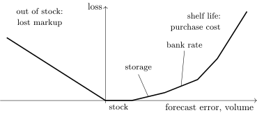
A piecewise-linear asymmetric loss function in sales forecasting. A shortage costs the lost markup; a surplus first costs storage, then the money frozen in the goods instead of a bank deposit, and when the shelf life runs out, the whole purchase cost. The slopes of all the pieces are measurable economic quantities.
Remark (Where the slopes come from). In the lecture someone asked: if the loss function has a dozen parameters, does choosing them not become a separate optimization problem? No. Only the model is optimized; the loss function is always given. All its slopes can be measured. How much it costs to store a volume of goods in a warehouse is a known quantity. If you overbought goods and froze money in them that could have been put into circulation or at least into a bank, the slope of that piece is the bank rate. If you overbought so much that the goods started to spoil in the warehouse, you lose their purchase cost, and that is known too. That is, in a well-run business these quantities are known. The other thing is that when we began applying this approach in practice, it turned out that although these data are known and updated, they often do not match reality and go stale, and since they do not critically affect the business process, managers are not especially motivated to keep them clean. When this came to light, both we and the client realized that the business processes ensuring clean data, including the auxiliary data needed to build the functional, had to be put right first. Generally speaking, one has to compute the total cost of restructuring the business processes and compare it with how much the increase in model accuracy will cut costs. The calculation of whether an implementation is economically worthwhile rests precisely on these data being collected carefully; until they are, the estimates have to be rough.
I will not go through ranking problems now — I have many examples, but there will be a special lecture on that.
Complexly structured data and deep learning
Not long ago machine learning moved on to solving, at scale, problems with complexly structured data, where there are no ready-made feature descriptions of objects. Let us return to the churn problem. It is interesting because the source data about customers is complexly structured: it is events in time. Here the customer took an incoming call, here they called themselves, here they changed the tariff plan, here they put money on the account, here they were online and traffic was flowing. A huge amount of diverse data about the customer's behaviour, but complexly structured and distributed in time somehow. Hence the problem: how to compute features from this raw data?
Very different data can be complex: text, a sequence of symbols; a signal, a continuous-valued sequence; an image, a 2D or 3D matrix; video; transactions, interactions of objects with one another; and all of this together. For such problems deep neural networks that can vectorize data automatically are used more and more. This first appeared in statistical machine translation, in speech-to-text and text-to-speech, in computer vision, and all these applications share one main idea: complexly structured data has to be turned into a vector of fixed dimension — a feature description of the object. With this vector machine learning already knows what to do.
If the features are computed by formulas a person came up with, this is feature engineering. If, however, the vectorization of an object is itself a model with parameters ,
then it can be trained jointly with the model that solves the problem:
This is feature learning. This is what deep neural networks really are — learnable vectorization of data, a complex superposition of functions that turns complexly structured data into a vector — and not at all that they resemble the human brain: that is not so important. What is important is that they fully automate the stage of feature generation, which used to be done only by hand: whole departments of engineers sat and invented features for each problem. Now there are models that seamlessly join vectorization with the classification model. This is the essence both of the problems we talked about and of dozens of others now called «Big Data». We will start talking about this next semester.
Peculiarities of the data and of the statements of applied problems
One more conceptually important thing. We often say that we deal with non-standard problems of function approximation. Function approximation has been known for ages: Carl Friedrich Gauss invented the method of least squares at the end of the 18th century, when he computed the elliptical orbits of planets from astronomical observations — the method is already more than two hundred years old. What, then, is non-classical about our problems? That the data, unlike in the problems mathematics has dealt with for two hundred years, can be:
- heterogeneous — features measured in different scales;
- incomplete — not all features measured, with gaps;
- inaccurate — measured with error;
- contradictory — identical objects, different answers;
- excessive — extremely large, not fitting in memory;
- insufficient — fewer objects than features;
- complexly structured — no feature descriptions.
Machine learning has learned to work with all these peculiarities and difficulties. It is, as it were, the next step in the theory of function approximation, but more practice than theory: all these peculiarities are present in one combination or another in every applied problem.
What machine learning cannot do is work with dirty data. Dirty data is lies in the data. Garbage in, garbage out — and nothing can be done about it. So in every problem one has to check with the client where the data comes from and how the human factor may affect its quality for the worse. The second cause of mess in applied research is a vaguely formulated criterion of model quality: the client wants a miracle from artificial intelligence but cannot say exactly which measurable indicator will characterize the quality of the forecasts or of the automation in their business process. Without that, embedding artificial intelligence anywhere is impossible.
Once again: every problem must have its DNA — given, find, criterion. This is my favourite formulation, and I repeat it very many times, especially when I begin working with clients: one has to find out at once whether they understand it or not. Twenty years ago it was widely not understood, and the conversation with each client had to start from exactly this point. Now things are much better, and as a rule people understand that no good predictive models can be built without data and without data quality.
The CRISP-DM standard and the evolution of artificial intelligence
The cross-industry standard for data mining CRISP-DM (CRoss Industry Standard Process for Data Mining) is an old thing, from 1999, and it was already old when it appeared: this whole business process of solving data analysis problems was well known from Soviet textbooks of the seventies. Five initiating companies — SPSS, Teradata, Daimler AG, NCR Corp. and OHRA — got together and decided to bring in at least some unification; back then there were not even such words as Data Science. The steps of the process:
- understanding the business that generates the data;
- understanding the data itself — where it is dirty, incomplete, inaccurate, heterogeneous;
- data preparation and feature engineering — bringing the data into a form convenient for modelling;
- model development and parameter tuning — the actual main subject of our course;
- quality evaluation — we will talk about that too;
- deployment — embedding the model built into a real business process, so that it works and is useful.
The evolution of artificial intelligence is conveniently understood as the automation of the steps of this scheme.
- Expert systems: rigid rule-based models. When artificial intelligence began in the fifties and sixties, machine learning appeared almost at once, but more hopes were then pinned on expert systems: how to play draughts? Take grandmasters, ask them the rules they use, and program those rules into the computer. This approach has been almost entirely displaced by machine learning; rule systems have kept niche applications.
- Machine learning: parametric models trained on data. Instead of tormenting experts, we take data and build predictive models that in effect emulate the decisions of a doctor, a credit analyst and so on. As a rule, machine learning makes decisions better and more reliably than people. It brought automation of the modelling stage.
- Deep learning: models with learnable vectorization of data. This is the seamless joining of two stages — preparing features from raw data and the model itself — into a single neural network, which turns out deep and which we train as a whole.
- AutoML: automatic choice of models and neural network architectures, seamless joining of modelling and evaluation, so that the computer itself goes through models, chooses by cross-validation and understands when there is already a reliable justification for switching from an outdated, worse model to a new, better one.
- Lifelong learning: all of this also works seamlessly in the production loop. There is no need to run around with terabyte disks carrying data from the production system to the test one and then the models back — in real enterprises that is a complicated organizational and bureaucratic process. A fully automatic system that itself chooses the best models should work right in the loop.
Clearly the wave of automation will continue to spread across this diagram, which is what we are seeing. Perhaps this view will help you choose what to work on: AutoML and lifelong learning are topics that, by all appearances, will be very important in the coming years.
Experiments in machine learning
When you develop new machine learning methods, or solve problems that have been solved thousands of times before you, or perhaps never by anyone, it matters how you run experiments. There are experiments of different kinds.
Experiments on a particular applied problem. The aim is to solve it as well as possible. Here understanding the problem and the data matters, and inventing informative features matters. This is how data analysis competitions work, for example on kaggle.com.
Experiments on a set of applied problems. The aim is quite different: you have developed a new method and need to try it on dozens or even hundreds of diverse problems and show that it works better than everything done before you. This is getting harder and harder: twenty years ago one could still compete like this, but now breakthrough results in new models are very hard to achieve, though many people still do such research. There are repositories of real problems — the main one in the world for such experiments is the UC Irvine Machine Learning Repository. Here you are not interested in the applied essence of each problem; you need not even think about its meaning: there is data, there is a criterion, and there are a few dozen such problems, with no time to think about each as an application area. The features, as a rule, have already been invented by someone.
Experiments on synthetic data — for developers of new methods. The advantage is that we know the true dependence (ground truth). The aim is to debug the method and find the limits of its applicability: to show that when the hypotheses and heuristics built into the model hold, the implementation works well and as intended. The objects are drawn from an invented distribution, often two-dimensional so that the sample can be visualized; the answers are for an invented function .
Experiments on semi-synthetic data. From synthetic data one has to move gradually to real data. Where in nature have you seen purely Gaussian distributions? They do not occur in nature. So let us take real objects: our method must be able to work on real . And let us set the answers ourselves, for an invented function, possibly with noise: after all, we are doing function approximation, and we need to understand how well the model can approximate all sorts of functions — which ones well and which badly. Remember the Runge example: hat-shaped functions should not be approximated by polynomials.
Summary
- The basic concepts of machine learning: object, answer, feature, loss function, model, learning method, empirical risk, overfitting.
- A problem statement is its DNA: Given, Find, Criterion.
- The stages of solving machine learning problems:
- understanding the problem and the data;
- preprocessing the data and inventing features;
- constructing a parametric model;
- reducing learning to optimization of the parameters;
- solving the problems of optimization and overfitting;
- testing, quality evaluation;
- deployment and operation.
- There are very many applied machine learning problems, they are very different, and they exist in every area of business, science and industry.
Remark (Overfitting and deep neural networks). After the lecture someone asked: have deep networks solved the problem of overfitting, or has everything stayed as it was? They have had an effect — in the sense that overfitting in deep neural networks turned out to be such an enormous problem that considerable research effort had to be spent on solving it, and fortunately it led to good results. We have learned to build models with billions of parameters from a comparable amount of data. It used to be thought that there should be several times, or better an order of magnitude, fewer parameters than data, and this belief weighed on mathematical statistics throughout the 20th century. Now that is no longer so: the development of deep networks led to successful methods of overcoming overfitting. Some of them — regularization and a few other techniques — are more or less understood, while why others work, including those related to choosing the network architecture, we do not fully understand.
A very important thing here is the shape of the landscape of the functional being optimized. Twenty years or so ago it was thought that a neural network is hard to train because the functional has many local extrema. Later it was found experimentally that this is not so: there are many local extrema, but they are roughly equal in quality; they can form manifolds, complicated ravines; and the shape of these ravines matters — one should look not only for deep but also for wide extrema, stable under changes in the composition of the data. Such a simple device in the design of a network as skip connections turns out to simplify the landscape greatly: a functional with many local extrema becomes smoother, with a large deep extremum. The optimization landscape is tied in a nontrivial way to the effects of overfitting, and building a unified mathematical theory that ties it all together is an open scientific problem today.
There is a mathematical basis, though: very deep theories are developing alongside practice. Conferences that twenty years ago were almost entirely about generalization ability and overfitting are now devoted to giving a theoretical answer to the question of why deep networks work, and how to make them better or more economical — for example, to cut the number of parameters by three orders of magnitude without loss of quality. This seems possible: today's enormous network sizes are brute force; people did what could be done quickly, and now the subtleties have to be worked out. When a single training run of a large language model requires tens of thousands of graphics cards and tens of millions of dollars, only a handful of corporations can afford it, while an average university cannot. How to invent economical deep network architectures, literally to reduce the cost of training them in roubles or dollars, is a mathematical problem and a very important topic for research.
No comments yet
Be the first to share your thoughts.