September 22, 2026 · Lecture · LibreTimes
Topology 2. Lecture 3
We will recall simplicial homology more than once, but now we finally study what is usually meant by homology: the singular homology of topological spaces. It is the generally accepted notion: it is assigned to any topological space and behaves especially well for CW complexes and spaces homotopy equivalent to them. We are gradually starting to study its theory: we will prove theorems about it, rigorously prove homotopy invariance, and understand how to compute it.
Singular chains
We will need some constructions with standard simplices. Let us fix: is the most standard simplex, the convex hull of the very specific points in , the standard vector space with these vectors as a basis. Its vertices are numbered from to , so for any subset of vertices there is a distinguished embedding of the standard simplex of smaller dimension into as a face. Let us fix such embeddings for the facets.
Definition (Standard inclusion of a facet). For the inclusion of the -th facet is the linear map taking in order to :
Its image is the convex hull of all basis vectors except : the facet opposite the vertex .
In general: if is a subset of cardinality , then, numbering its elements in increasing order, we get a linear map , , a homeomorphism of onto the -dimensional face . The inclusion of a facet is the case : opposite a vertex stand all the others; I order them increasingly and take the order-preserving bijection with the vertices of .
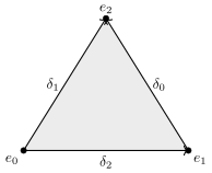
and its three facets. The arrow shows how the standard segment is included: from the image of to the image of . is the facet opposite vertex , opposite , opposite .
Definition (Singular simplex, singular chains). A singular -dimensional simplex of a space is a continuous map . The group of -dimensional singular chains is the free abelian group generated by the set of all singular -simplices of ; for we put . The differential is given on the basis by
The homology of the complex is called the singular homology of the space : .
The word "singular" means that the map may have singularities: it need not be smooth, it may intersect itself, it maps however it likes. The composite is a singular simplex of one dimension less, so the formula makes sense. Sometimes one writes in more detail : the restriction of to the facet spanned by all vertices except the -th. This should be understood as informal notation: the restriction of to a facet is a map from the facet to , whereas we need a map from the standard simplex ; a facet of the standard -dimensional simplex is not the same as the standard -dimensional one, and one also needs the composite with the standard homeomorphism between these two convex sets. The rigorous definition is via .
As usual, one has to check that we get a chain complex, but the check is the same as last time, and I will skip it. follows from the simplicial identities: including a facet and then including a facet again is the same as removing first the -th vertex and then, from what is left, the -th, with a correction for the index shift; the signs change so that everything cancels. It is clear anyway: if you ignore the signs and apply the differential twice, you get a sum over all faces of codimension two, each face counted twice; the signs are chosen so that these pairs cancel.
Remark (an important disclaimer). A singular -simplex is, of course, a path from one point to another. There is also the opposite path, traversed in reverse order. Intuitively one very much wants to say that in the group of chains they are opposite. No: they are simply different basis elements of . We do not quotient by any orientation relation. A reparametrisation of a path also gives a different basis element. At the level of homology this leads to the same thing, but why is a separate story: one has to map some little triangles in accordance with the reparametrisation. At the level of chains these are completely different elements of a very big free abelian group. In the same way, if the faces of a simplicial complex are regarded as singular simplices, then before we had only them, and now the "opposite" ones have appeared as well.
Zeroth homology
Let us start with the little that can be computed, zeroth homology; it can be described completely: it corresponds to the path components.
Theorem (Zeroth homology).
- If is path-connected, then .
- If is the decomposition into path components, then for all ; when computing homology one may assume path-connected.
- For any the group is free abelian with a basis in bijection with the set of path components.
Obviously 3 follows from 1 and 2.
Remark (on dimension). Formally, for the simplex is the empty set, there is exactly one way to map the empty set into , and should be . Geometrically this is meaningless: go to a geometer and tell them that the empty set is a polyhedron; with this approach the dimension of the empty set is , while some consider it . So by definition for . The positive ones are all there: if is nonempty, a simplex of any dimension can at least be mapped to a point. If one does use this formal point of view, one gets reduced singular homology; more on it below.
Proof. Part 1. The complex ends like this: , so . The group is the free abelian group spanned by the points of ; I will denote it (I very much like this notation; square brackets must on no account be used here: they are taken by homology classes). Its elements are formal finite linear combinations of points: twice this point, minus five times this one, seven times that one.
Let be a path. By the formula for the differential: the facet opposite vertex gives the point with a plus sign, the facet opposite vertex gives the point with a minus sign:
The boundary of a path is the difference of the two points it connects. So is the subgroup generated by the differences over all pairs of points connected by a path. If is path-connected, these are all pairs:
This group is isomorphic to by the homomorphism theorem: consider the augmentation sending each point to one. It is surjective, and its kernel is exactly the subgroup we quotient by (an easy check). So .
Geometrically everything is very simple. As a generator one can take the class of any point: a point is a zero-dimensional chain and a cycle, so the notation makes sense, and for any two points, because there is a path whose boundary is their difference. All in accordance with the familiar: homology is classes of cycles up to boundaries of chains of one dimension higher. Altogether is the free group on one generator.
Part 2. The image of a simplex under a continuous map is path-connected, so it lies in a path component, and a unique one: for each there is a unique with . The basis of has split into a disjoint union of the bases of the groups , and
The differential is compatible with this decomposition: the restriction of to a facet lands in the same component. So the complex is the direct sum of the complexes with the direct sum of the differentials, and the homology of a direct sum of complexes is the direct sum of the homologies (I think this was a problem). Everything follows from the fact that the simplices map into different components.
Here is an example of topological information that gets lost. Consider the sine curve together with the vertical segment it accumulates on: this is a connected but not path-connected space, and , because there are two path components – the curve and the segment.
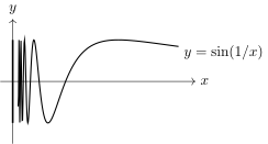
The topologist's sine curve: the graph of for and the segment it accumulates on. The space is connected but not path-connected; .
The homology of a point
An important computation, essentially the only one we will do: the point is the only space (besides the empty one) for which we understand well what its chains look like. The zeroth homology of a point is , we know that. A point has no other homology.
Theorem (Homology of a point). , for .
Proof. is the free group with a single generator : the map of all of to the point. The restriction of to any facet is a map to the point, that is, , so
(a very hard computation: , with terms). The chain complex is written out explicitly:
the arrows alternate: from even degrees goes an isomorphism, from odd ones zero. Cycles: the kernel of an isomorphism is zero, the kernel of the zero map is everything, so for odd , for even , and , an artefact of the end of the complex. Boundaries: the image of an isomorphism is everything, the image of zero is zero, so for odd and for even. The quotient: for odd it is , for even it is , and the only nonzero group is .
Reduced homology
Definition (Reduced singular homology). The complex of reduced singular chains differs from by one group: , the free group on the unique map , with the differential being the augmentation that sends each point to one. Its homology is the reduced singular homology of .
This is how the reduced homology of any space is computed. For a point, one more copy of is added to the complex in degree , and the arrow is an isomorphism: the alternation continues one more step, and all the reduced homology of a point is zero; also useful to remember; it is an exercise.
Remark (why two versions). Why is kept in degree zero in ordinary homology? So that for Cartesian products of spaces the homology multiplies by tensor product, and so that for disjoint unions zeroth homology behaves correctly, as in part 2 of the theorem: a disjoint union of points has reduced homology (check it). Both versions are useful in different constructions.
The intuition one of the students came up with ("ordinary homology is a good functor from topological spaces, and reduced homology from pointed spaces") does not quite work. For pointed spaces one should consider relative homology; it is isomorphic to reduced homology, but reduced homology is defined for spaces without a basepoint, and it is important to understand this: reduced homology always exists, and there is no basepoint in it, which is mysterious. On the other hand, it gives an elegant way to state things like "homology like that of a point up to dimension ": for ; such a space is called homologically -connected. Another formulation from the audience: ordinary homology preserves colimits from the category of topological spaces, reduced homology from the category of pointed spaces.
That is enough for a first acquaintance with homology.
Chain maps
Everything we have defined so far are objects. Basic knowledge: one cannot do without categories; besides objects one must consider maps between them. We know how to map topological spaces, but not yet chain complexes and homology groups. Let us learn.
Definition (Chain map). A chain map between chain complexes is a family of homomorphisms for all that commute with the differentials: , that is, the diagram
commutes.
A composite of chain maps is a chain map: put two such diagrams side by side and erase the middle arrows; you get commutative rectangles, and a rectangle is the same as a square. The identity map is, of course, a chain map. So chain complexes and chain maps form a category.
Theorem (A chain map induces a map of homology). A chain map defines a homomorphism for each (a graded homomorphism ) by the formula
Moreover, and .
Proof. The down-to-earth proof. Every element of can be written as , where , , possibly non-uniquely. First, , so is a cycle in and the notation makes sense. Second, well-definedness: if , there is with ; then
again by the chain property of ; that is, and differ by a boundary and define the same class. The answer does not depend on the choice of representative, the formula defines a well-defined map of sets, and it is easily checked that it is a homomorphism.
The clever way. contains the subgroup of cycles (the kernel of the differential) and the subgroup of boundaries (the image); likewise in . The image of cycles consists of cycles, the image of boundaries of boundaries: if , then ; if , then . So restricts to and takes into . And then a general fact from algebra – the universal property of the quotient group: a group homomorphism taking a normal subgroup into a normal subgroup defines a unique homomorphism of the quotient groups making the diagram commute. That is exactly , with the same formula.
Functoriality (a composite induces the composite, the identity the identity) follows from the formula.
So taking homology is a functor from the category of chain complexes to the category of graded abelian groups. That is how we passed from homological algebra to algebra. Now – from topology to homological algebra.
Theorem (A continuous map induces a chain map). A continuous map defines a chain map
(on the basis; extended by linearity). Moreover, and .
Theorem (Corollary). A continuous map induces a homomorphism for each ; , .
Proof. The construction is very simple: composing a singular simplex with gives a singular simplex ; on an arbitrary chain the value is (I will not write this any more: a homomorphism from a free group is given on a basis). We need to check that this is a chain map, that is, :
We got the same thing, because composition is associative. All such formulas follow from associativity; for the identity map too. The corollary is the composite of two functors.
Summary: we have three functors,
from the category of topological spaces and continuous maps to the category of chain complexes of abelian groups and chain maps, from there to the category of graded abelian groups and graded homomorphisms, and their composite is singular homology. Instead of graded groups one can consider separately the functors into ordinary abelian groups.
Theorem (Corollary). If are homeomorphic, then for all .
For a homeomorphism this is, in principle, clear from the definition: everything was defined through the internal structure of ; and here we checked it explicitly through the associativity of composition of continuous maps. It is also true for a homotopy equivalence, but that we will prove with great effort.
Homotopy invariance
Theorem (Homotopy invariance). If are homotopic, then for all .
Theorem (Corollary). If are homotopy equivalent, then for all . In particular, if is contractible, then and for , which is not at all obvious from the definition.
The corollary is derived from the theorem by general facts about homotopy equivalences: if and , then the composites are homotopic (this follows from the transitivity of the homotopy relation), so the category whose morphisms are homotopy classes of maps is well defined, and a functor taking homotopic maps to equal ones takes a homotopy equivalence to an isomorphism. Whoever does not understand how this corollary is proved – check it from the definition, and you will understand better what a homotopy is.
On to the theorem. At the level of chains, homotopic maps of course induce different maps: I moved the map smoothly, and a simplex that was mapped here is now mapped there – a completely different basis element. But they are also homotopic in some sense: there is a good algebraic analogue of the notion of homotopy.
Definition (Chain homotopy). Let be chain maps. A chain homotopy between and is a family of homomorphisms , raising the degree by one, such that
If a chain homotopy exists, and are called chain homotopic: .
The meaning of this definition is not visible now; by the end of the lecture it will become clear; if you take the exam, you will have to memorise it, but for now it is enough to understand it. The geometric motivation: is for prism. From a simplex we make a prism. The boundary of the prism consists of two lids and the lateral surface, and the lateral surface is the prism over the boundary of the simplex:
that is, , exactly that formula. The signs: one lid with a plus, the other with a minus, because the outward normal sticks up at one and down at the other, and we draw everything from bottom to top.
Remark (graded commutator). One would like to be a commutator; and it is one, but in the graded sense. In graded algebras the commutator of homogeneous elements is defined as . The degree of is , the degree of is , so . The differential can be thought of as a map of degree : from to .
Lemma (Chain homotopic maps are equal on homology). If , then .
Proof. The check is very simple. Every element of is the class of a cycle . A difference of cycles is a cycle, so
here , and the class of any boundary is zero. That is the end of the proof: the magic formula works and gives equality of the classes.
Now the saddest part of the lecture: the proof of the theorem.
Proof. Let be a homotopy, , . We want to build a chain homotopy with
then by the lemma.
The idea. Over there is the cylinder : the bottom base maps to by , the top by , and the whole cylinder by . From a singular simplex we want to make a linear combination of -dimensional singular simplices in . What can I build? Multiply by a vertical segment and map the prism:
One must match desires with possibilities: all I can do is a singular prism in . And I want not a prism but a linear combination of simplices. So the prism must be cut into simplices.
The standard subdivision of the prism. Denote the vertices of the bottom base by , and of the top by . For a set of vertices of the prism, denote by the linear map , . The prism over a segment is cut into two triangles, and ; the prism over a triangle into three tetrahedra,
(this was a problem on the first sheet). The scheme: I walk along the bottom vertices in order, at some moment decide to go up, and then walk along the top ones. In general
and this really is a subdivision of the prism into simplices. If anyone does not see it, buy some cheese, take a knife and do it. Actually, that this is a subdivision does not even matter to us: what matters is that we believe that if we take a linear combination of these simplices with the right signs, the boundaries will cancel and the top lid, the bottom lid and the lateral surface will remain. The lateral squares are cut by diagonals according to the same scheme. We did not orient anything – I just ordered the vertices, and that automatically gives an orientation: the arrows from the smallest vertex to all the others form a basis; restricting to a facet with the induced order gives the same thing.
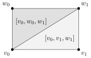
The prism over a segment and its subdivision into the two triangles and .
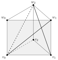
The prism over a triangle . The thick edges are the diagonals , , , cutting it into the tetrahedra , and ; the front square is cut by the diagonal , the back ones by and .
Remark (lattice paths). The simplices of the subdivision are enumerated by lattice paths in the grid from the bottom-left corner to the top-right: a step to the right means the next vertex in the same base, a step up means passing from to . In exactly the same way the product of any two simplices is subdivided into simplices – by lattice paths in the grid, and there are as many of them as there are shuffles. Why the simplices cover the whole prism and do not intersect in their interiors we do not need, and it is part of a problem on the first sheet.
The definition of . Finally,
The composite is always the same from here on, so in the computation I will informally write just the bracket , meaning this composite. All the differentials work by deleting the -th vertex from the bracket with the sign . It remains to compute; it will not be very pleasant, and following it is even less pleasant, but it is useful to realise it for yourself at least once in your life – though in principle not necessary, because the geometric picture has already been given. What follows is an exercise in carefulness: how the operator of deleting a vertex commutes with the "doubling" operator .
Computing . In the bracket the vertex stands in position , and in position (because of the doubled index ). Four types of vertices can be deleted:
The two middle terms give a telescoping sum: for it is , for it is , and so on up to : ; everything cancels except
the restriction of to the top base is , to the bottom , so and . Denote the two remaining sums
so that . It remains to see that .
Computing . , and to each , a simplex with vertices , one has to apply the same procedure: walk along its vertices up to some vertex inclusive, writing , double it as , and then write . The jump can be made before or after :
in the second sum there is an index shift: in the simplex without the -th vertex, the vertex for stands in position . Altogether
The first sum is exactly (the same brackets, the sign against ), the second exactly (the sign against ).
The result.
that is, . It all works out.
Perhaps it is more useful to work through it yourself; I more or less drew it for the triangular prism.
The homology of a pair
Ten minutes left; I wanted to start with this, but perhaps it is more useful for you to think about it a little earlier.
Definition (Subcomplex and quotient complex). A chain subcomplex is a family of subgroups that survive the differential: . The inclusion is an injective chain map. The quotient groups acquire the structure of a chain complex with the differential (an exercise; square brackets are inconvenient for cosets because they are taken) – the quotient complex .
This is a problem on the sheet; one can compute the homology of such quotient complexes.
Definition (Homology of a pair). If is a subspace, then is a subcomplex: this is not a definition but an obvious statement: if a simplex lands in , then so does its restriction to any face. The homology of the quotient complex
is called the relative homology of the pair .
The notation has a comma, not a slash: this is not the homology of the quotient space .
I will not explain the geometric meaning in detail now, but the idea is this. There is a space and a subspace on which I do not really care what happens. I take some thing – a linear combination of singular simplices – whose whole boundary lands in ; if is ignored, I as it were see something without boundary. Such chains define relative homology classes. In particular, a manifold with boundary mapped into so that the whole boundary lands in – that is roughly how one can think about relative homology classes. Next time we will study them.
No comments yet
Be the first to share your thoughts.