September 22, 2026 · Lecture · LibreTimes
Topology 2. Lecture 2
Contents
- Topological data analysis
- Persistence modules
- The structure theorem and the barcode
- The Vietoris–Rips and Čech complexes
- Stability of the barcode
- The Hausdorff and Gromov–Hausdorff distances
- The Wasserstein distance between barcodes
- The nerve theorem
- Covers and the nerve
- The category of covers and paracompactness
- Two more notions in terms of covers
After the introduction to simplicial homology, let us talk about where it shows up in real life. In the course itself simplicial homology may come up again, but only sporadically: we will mainly study singular homology, and the next lecture will be devoted to it, not this one. But simplicial homology is useful in topological data analysis – a field which, like the guinea pig (which is neither a pig nor from Guinea), is neither topology nor data analysis in the usual sense, but has something of both. We will start with that, and then talk about related mathematical topics: the nerve theorem and what can be defined in terms of covers. It will be a general-education lecture.
Topological data analysis
Data is a large finite set of points in a space of, say, very high dimension; there is a distance between them. I chose the letter because these will be the vertices of a simplicial complex. We want to analyse the shape of this set, the shape of data. What is meant? Suppose I am given many points in the plane, and I believe that they lie on a circle: the points are sampled, a sample of independent identically distributed random variables with a distribution concentrated near some manifold. One expects this manifold to be interesting, some nontrivial topological space. In the plane we see it with our eyes, but in reality there may be a hundred thousand points in a space of dimension a million. There are dimension-reduction algorithms: distorting the distances slightly, lower the dimension of the ambient space and then draw plots. The idea here is different.
It is pointless to study the topology of a discrete set; it is trivial. So we replace each point by a ball of small radius and consider the space
the union of balls of radius centred at the points of ; whether they are open or closed does not much matter. The balls are taken in the ambient space; in general can be replaced by any metric space in which is embedded; there are different metrics.
If is very small, this is bad: is homotopy equivalent to a discrete set of points. If is too large, it is also bad: the neighbourhood of the set is contractible, the points stick together into one big ball, we are looking at them from afar. So we want to look at intermediate values; in our example, for a suitable the union of the little balls reflects quite well the topology of the circle near which the points lie. But it is not known in advance which value to take; so we have to consider all values at once. (A question: what if the dynamics of the topology in is itself interesting? It can be interesting too, but the original idea is that there is a "right" , neither too large nor too small.)
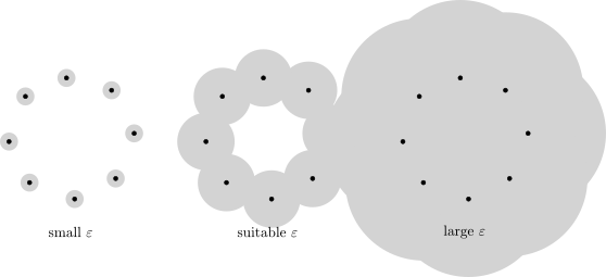
Points sampled near a circle, and for three values of : a discrete set, something like a circle, a contractible blob.
Persistence modules
In this course we study homology, and we will understand that to each topological space there corresponds a family of abelian groups, its homology groups, and to maps of spaces there correspond homomorphisms of homology groups. Homology is what can actually be computed. So let us consider the homology of each of the spaces for all . Together they form what is called a persistence module.
Definition (Persistence module). A persistence module is a family of abelian groups , one for each , and homomorphisms for all , compatible with one another: the homomorphism is the identity, and the composite equals .
It is something like a chain of groups and homomorphisms, only a chain is as it were the integer points of the line, while here there is a group for every real point of an open ray: a continuum of data.
This is exactly what happens with the homology of unions of balls. If , there is a natural inclusion , and we will discuss why it gives a homomorphism : we will prove that any continuous map of topological spaces induces a homomorphism of homology groups. Compatibility follows from the fact that taking homology is a functor: the inclusions form a commutative diagram, and a functor takes a commutative diagram to a commutative one. For simplicial homology we have not discussed this; it is a problem on the sheet; it is a rather nontrivial topic: even changing the order of the vertices is nontrivial, the simplices have to be multiplied by the signs of permutations.
So to a set of points we have assigned a persistence module. How should we picture it and what should we do with it? It turns out that the algebraic structure here is rather simple if homology is computed with coefficients in a field; over the integers everything is more complicated. We simplify: bring it to a canonical form.
In practice the set is finite. For each moment of time there is its own space, and their topologies differ: first five points, then five balls, then five balls two of which intersect, then something else, then everything has stuck together. But it is clear that the homotopy type changes finitely many times: if is finite, the homotopy type of changes finitely many times. We will prove that homotopy equivalent spaces have the same homology, so up to a critical moment, when two balls touch, the homology does not change. Hence the persistence module also changes finitely many times: there are critical moments when some balls begin to touch, and only at those moments does something happen. So one can think not of a continuum of data but of a chain of groups and homomorphisms
where to each group is attached the moment of time at which it is taken. We will call such persistence modules piecewise constant (the word was chosen by vote: "of finite type" does not fit, that name should go to modules in which each group is finitely generated). We start the process of inflating balls around the points under study; in the end we will get a contractible space, but before we get it, many interesting things will happen.
The structure theorem and the barcode
Now let homology be computed with coefficients in a field , so that all the are vector spaces over . The obvious persistence modules one can think of: zeros everywhere; then at some moment a one-dimensional module is born; then it maps isomorphically to itself; at some moment it dies, and there is nothing more. It could be born and die at once, and it could never die.
Definition (Interval module). For the interval module is the persistence module with for and otherwise, all maps between nonzero terms being identities.
The half-open interval, open at one end and closed at the other, is a convention: which one depends on whether our balls are open or closed. In the general case, when there is no piecewise constancy, one has to consider closed intervals, open intervals and half-open intervals of both kinds.
Theorem (Structure theorem). Every piecewise constant persistence module over a field with finite-dimensional is a direct sum of finitely many interval modules .
A module that never dies is, for example, zeroth homology: it never dies; in our example all the others, of course, die.
There are two proofs. The first: such a chain of -modules and linear maps is a graded module over the polynomial ring in one variable. If all the maps are denoted by one letter , then a polynomial, say , acts on an element by definition as . The polynomial ring in one variable over a field is a principal ideal domain, and then one uses the structure theorem for finitely generated modules over such rings, in the graded version, since the isomorphism must preserve the grading. (Someone in the audience noted that the ordinary structure theorem does not preserve the grading and that the indecomposable representations of the quiver are not arranged the same way as graded ones; the lecturer put the reference to the structure theorem in quotation marks: for graded modules over graded rings of principal homogeneous ideals "there is something along these lines", and one can also approach it through the theory of quivers.)
The second proof: an explicit algorithm, first-year linear algebra. We go by induction along the chain from left to right. We draw each module as a strip, increasing; having lived to the moment , we already believe that up to this moment the module is a direct sum of interval modules: each strip is a one-dimensional module that was born at some moment and perhaps died. At the moment we have a finite-dimensional space with a basis of those who have survived, sorted by time of birth, the earliest born first. At the next moment appears and a linear operator , an matrix. I want to bring to diagonal form, with some ones on the diagonal, then zeros, and everything else zero, that is, to Smith normal form: then some strips will survive, some will die, and the picture will again be as before. What is allowed?
- Changing the basis in arbitrarily, that is, any row operations: nothing has been decomposed there yet.
- In , replacing by , that is, adding to a basis vector those born before it. The strips are direct summands of the module up to the moment ; if you add an older generator to a new one born at some moment, the whole chain up to that moment can be left as it was: the decomposition up to does not change. These are column operations: previous columns are added to a column.
Take any matrix . By elementary row operations bring it to reduced row echelon form. Then add to each column the previous ones with the right coefficients and wipe out all the asterisks; we get a diagonal matrix of ones and zeros. That is all. It is not necessary to memorise this, but it shows that everything works.
This is the case of piecewise constant modules with finite-dimensional groups. People have also dealt with the general case, with neither piecewise constancy nor finite-dimensionality, but still over a field; similar theorems work there too; in practice everything is finite-dimensional and piecewise constant.
Conclusion: every such persistence module over a field is a direct sum of modules , and it can be drawn: to each summand corresponds a half-open interval from to , that is, a segment, a ray or a point.
Definition (Barcode). The diagram in which the persistence module is depicted by the family of half-open intervals is called its barcode.
A bar is a line, and a barcode is literally the striped code you see at the airport. Where the word "persistent" comes from: persistence, stability in the sense of "you are not going anywhere".
In the example where points are scattered near a circle, one can compute the homology of the spaces that arise. First the points gradually stick together, then they stick together into something like a circle (I am describing the homotopy type), then everything sticks together into a point. Let us follow the zeroth homology: at first as many copies as there are points; eventually one survives, and the rest die – some earlier, some later. There is also first homology. We will find out that of the circle is , while a contractible set has trivial first homology. So at some moment a circle was born, and it lives until everything contracts to a point.
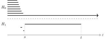

The barcode of a point cloud near a circle. In there are as many strips as points: all but one die quickly, one lives forever. In there is one long strip (the circle, born at the moment and contracted to a point at the moment ) and short junk ones.
If you scatter many points near a circle and carry out this procedure, you get junk data, which should be ignored, and data valuable to us, features, which we believe to be something meaningful. Clearly, the larger , the greater the chance that it is not junk. If the points are scattered on a circle of radius , the length of the strip of first homology will be roughly , while the length of the junk strips will be roughly the distance between neighbouring points. When there are many points, is small and decreasing, while stays; with a trillion points almost no junk will be visible.
So the pipeline is: a finite set of points ; from it a filtered topological space, a chain of spaces nested in one another; its homology forms a persistence module; from it one gets the barcode :
The barcode is already a purely finite set of data, a set of real numbers: segments, rays and points. This is our feature, a tool that can be analysed, classifiers can be run on it, and so on.
Remark (persistent does not mean filtered). A persistence module is not a filtered module, and these notions should not be confused. A filtered module is a chain of modules that embed into one another; here the maps can have kernels, homology dies.
A question from the audience: how hard is it, in general, to track where the homology changes? The problem is that we do not know how to compute homology. At least you do not; I do, and I will now teach you to compute the homology of these unions of balls. The algebraic side of the barcode question more or less ends here.
The Vietoris–Rips and Čech complexes
Computing on a computer the homology groups of from the set and the distances between points is hard: we have a space glued from balls, and from it we still have to build something whose homology can be computed. The idea is to consider simplicial complexes instead of these spaces: the Vietoris–Rips complex and the Čech complex. It turns out that the homology of is the same as the homology of the Čech complex; the Vietoris–Rips complex has different homology, but it is easier to compute, and in some sense it is close to the Čech complex. These are filtered simplicial complexes, and for them homology can already be computed: it is the simplicial homology we discussed.
Definition (Vietoris–Rips complex). Let be a finite metric space and . The Vietoris–Rips complex is the simplicial complex on the vertex set containing those sets of vertices whose points are pairwise at distance at most , that is, .
The axiom of a simplicial complex obviously holds. If is such that the distances between three points are all less than , we add the whole triangle; if a fourth point is also within of one of them, we add that edge, but not the edge to a farther point; if four points are close, I draw the whole tetrahedron.
As grows, the complex behaves similarly to the union of balls: embeds in for as a simplicial complex, and something happens in it: a tetrahedron appeared here, something else there. Where the union of balls had a circle, the points will join into a circle, but all sorts of silly higher-dimensional simplices will be added; you get a formation that is not even flat, it contains tetrahedra; it is an abstract simplicial complex, but one sees, at least intuitively, that it is homotopy equivalent to a circle. After a while it will again turn into a contractible polyhedron, and for very large the Vietoris–Rips complex is the whole simplex . The simplicial homology of this chain gives a persistence module: maps of simplicial complexes also sometimes lead to maps of simplicial homology; we have not discussed this yet.
It is clear how to compute this on a computer. Measure the pairwise distances between the points; the complex changes only at the moments when equals one of these distances. At each such moment, build the complex and compute its homology: you get a family of free abelian groups or vector spaces; bring the matrices to the right form, compute kernels and images, take quotients. The homology is computed – and so is the barcode. There is a program, Ripser (in Python), that does this from the pairwise distances or the coordinates of the points; it computes and easily, and after that it begins to struggle: as grows there are many simplices, and all of them have to be found. For zeroth and first homology it is enough to know which points, segments and triangles are in the complex; that is easier to store. In practice people work with , , , and that is enough for them. The coefficient ring is taken to be the field with two or three elements: that finds everything related to -torsion, and there is usually no -torsion, the topology is not that sophisticated.
Remark (names). Vietoris is the same as in the Mayer–Vietoris theorem. Eliyahu Rips is the one who worked on geometric group theory; you can hear about him in a course on geometric group theory.
This is the first combinatorial approximation to what happens with the balls. It is not the same thing (the homology of the Vietoris–Rips complex is not directly related to the homology of ), but it is also a persistence module, and one can also build a barcode. The second example, more expensive algorithmically: the Čech complex.
Definition (Čech complex). Let be a finite subset of a metric space and . The Čech complex is the simplicial complex on containing those sets of vertices for which the balls of radius centred at the points of have a common point:
To find out whether to add a triangle, one has to draw the balls and see whether they intersect all together. Three balls can intersect pairwise but have no common point; then the Čech complex has three edges without the triangle. Similarly one gets a persistence module of the simplicial homology of the Čech complexes and the corresponding barcode.
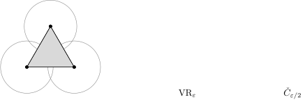
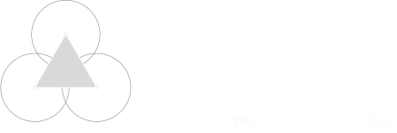
Three points at pairwise distance . The balls of radius intersect pairwise but have no common point: contains the triangle, the Čech complex built from these balls only its boundary.
Two constructions, both combinatorial approximations to the union of balls, both give simplicial complexes, and each has its advantages and drawbacks.
The Vietoris–Rips complex. Easier to compute; no ambient space is needed, only the matrix of pairwise distances, and that is already quite pleasant. Moreover, it is a flag complex: it is determined by its one-dimensional skeleton, that is, it is the largest simplicial complex with these edges. One can build it like this: take all the edges, glue in triangles wherever there is a complete graph on three vertices, tetrahedra wherever there is a complete graph on four, and so on.
The Čech complex. Harder to compute: an ambient space is needed, and one has to check whether a given set of balls has a common point, which is a combinatorially harder problem; I think one first has to compute the Voronoi partition and then look at the distances at its vertices, while for Vietoris–Rips nothing of the kind is needed. But it has a remarkable advantage.
Theorem (the Čech complex computes the homology of the union of balls). The geometric realisation of the Čech complex is homotopy equivalent to the union of balls:
This is a consequence of a general theorem, the nerve theorem; more on it below. That is, the Čech complex computes exactly the barcode we wanted.
The complexes are related to each other: if the pairwise distances between points are at most , then any of the points lies in all the closed balls of radius centred at them, and if balls of radius have a common point, the pairwise distances are at most ; altogether
The complexes are close to each other in some sense, so one can expect the homology to be close, and hence the barcodes to be close in some sense too. Note that everything depends on the metric: I draw Euclidean balls, but one can take the , , norms, and then these complexes acquire specific properties.
Stability of the barcode
One more topic from data analysis. We have built an invariant of a dataset; the question is how sensitive it is to changes in the initial conditions. This is a question of stability, and from the mathematical point of view of the continuity of a certain map. The pipeline can go through the union of balls, through the Čech complex or through the Vietoris–Rips complex; in fact practitioners, of course, compute Vietoris–Rips. So there is a map
assigning to a set of points its barcode (via Vietoris–Rips). It is just a map of sets. Is it continuous? Is it true that if you jiggle the points slightly, or add a new point close to one of the old ones, the barcode changes little? Can it happen that I moved a point a tiny bit and the homology immediately exploded?
The answer: no, the map is continuous. This is the stability theorem. In fact it is a theorem about being Lipschitz: if the metrics are introduced correctly, the map is Lipschitz. A clarification from the audience: it is not quite about the homology changing little; it is about the intervals on which it lives changing little. The homology itself may change a lot, but for an insignificant time, so that we do not have time to notice: many very short segments may have been added. What matters is one long segment: about it we will say "aha, there is something", and about short ones, "errors".
Theorem (Stability). For finite metric spaces ,
where on the left is the distance between barcodes (the -Wasserstein metric, also known as the bottleneck distance), and on the right the Gromov–Hausdorff distance between the finite sets we started from.
The definitions of these metrics are given by vote: nobody admitted to being a pure mathematician who does not want to get their hands dirty knowing the definitions of such things.
The Hausdorff and Gromov–Hausdorff distances
Definition (Hausdorff distance). Let and be compact sets in a metric space . The Hausdorff distance between them is
To remember the formula, a picture: I take the point of farthest from and the point of farthest from , and add these two distances. A pleasant problem: check that this is a metric on the set of all compact subsets of .
If, on the other hand, and are abstract compact metric spaces, not embedded anywhere, one can consider all possible ways of embedding them into some metric space and compute the distance between them there. Say, the unit disc and the unit square: how close can I place the disc to the square isometrically in some metric space? Most likely the closest will be when they are placed concentrically. This is the idea of the best overlay of one on the other in an ambient space, such that both map there isometrically.
Definition (Gromov–Hausdorff distance). For compact metric spaces ,
where the infimum is taken over all metric spaces and all isometric embeddings , .
Compact metric spaces do not form a set, but compact metric spaces of bounded cardinality, that is, those with at most points, do, and for any cardinal this metric makes them into a metric space.
This definition is impossible to work with in practice, but fortunately for finite sets there is an explicit formula.
Theorem (explicit formula for finite spaces). Let and be finite metric spaces. Then
where the minimum is over all correspondences between and , that is, subsets whose projections onto and onto are surjective.
A correspondence is a generalisation of a function: a multivalued function from to , as multivalued as you like, but defined everywhere and taking all values. The Gromov–Hausdorff distance is computed by going through all correspondences. The expression under the minimum is called the distortion of the correspondence : the pair of points has as it were gone to the pair , and I look at how much the distance has changed; ideally I want equality. The distortion measures how far is from being isometric: if is an isometric correspondence, the distortion is zero, and so is the Gromov–Hausdorff distance. We go through all correspondences and look for the one closest to an isometry. That is how different the metrics on my finite sets of points are.
The Wasserstein distance between barcodes
Now the metric on barcodes. I like to think of it in terms of economics; it came from optimal transport. The following problem is solved: given barcode number one, I want to make barcode number two out of it, spending as few dollars as possible. Allowed:
- moving an end of an interval by , spending dollars: replacing the interval by or ;
- adding and removing points (intervals of zero length) for free.
If one barcode has to be turned into another, I spend some dollars to shrink a superfluous segment to a point and some to move the ends of the others. Two segments, and , not far from each other: it is most profitable to move end to end, the distance is . Two segments far from each other: one can move one into the other, but it is unprofitable; it is cheaper to shrink both to points, and the distance equals the sum of their lengths. I may have got the constants slightly wrong (somewhere the rate may be twice as large), but mathematically that is a trifle: such a metric is natural on the set of families of segments. If the costs of the moves are added up, you get the -Wasserstein metric; if you take the largest of them, the -metric, the bottleneck distance, which is what appears in the stability theorem.
One more way to think about it. Consider a diagram in the plane with coordinates : each segment of the barcode gives a point above the diagonal. The closer a point is to the diagonal, the more it looks like junk. To a barcode we assign the union of the set of these points with the diagonal, a subset not even of the plane but of the extended plane : an interval that was born and will never die gives a point at infinity. This is a metric space in a generalised sense, with infinite distances. Then the distance between barcodes is more or less the same as the Hausdorff distance between these sets: points on the diagonal may be added for free, shrinking a segment to a point is moving the point towards the diagonal, and moving the ends is moving the point vertically or horizontally. Here it is exactly the Hausdorff distance, not Gromov–Hausdorff: the diagonal is fixed in the plane, moving it is forbidden. I ignore the fine points about multiplicities (whether points can coincide, whether it is a metric or a pseudometric), and I do not remember the precise statement of whether the Wasserstein distance between barcodes can be expressed this way.
This is one of the few genuine theorems in this science: the barcode is a Lipschitz invariant of a finite metric space; under small changes it changes little.
The nerve theorem
From here on we do mathematics. One theorem remains without proof: that the Čech complex is homotopy equivalent to the union of balls. I will not prove it anyway, but I will explain where it comes from: from the theorem on the nerve of a cover. The idea is that balls are convex, and intersections of balls are convex too; that is what allows the union of balls to be replaced by a simplicial complex. This is a notion of general topology, covers.
The theorem is called Alexandrov's nerve theorem, although in its present formulation it was, I think, proved by Borsuk; it is usually stated for paracompact spaces, and paracompact spaces were invented by Dieudonné.
Covers and the nerve
Our covers will be open: an open cover of a space is a family of open sets indexed by a set (which may be infinite) whose union is all of . In terms of covers one defines, for example, compactness: from any open cover one can extract a finite subcover; there is countable compactness and other weakenings. I, on the other hand, want to associate with a cover a combinatorial structure, a simplicial complex. This is Alexandrov's idea.
For a finite denote by
the intersection of the corresponding members of the cover. Some intersections are empty, some are not.
Definition (Nerve of a cover). The nerve of an open cover is the simplicial complex on the vertex set
This is a simplicial complex: if and , then is also nonempty. Finiteness of is required because we defined a simplicial complex as a family of finite sets.


A cover by four discs: neighbouring ones intersect, is shaded, . The nerve is a path on four vertices; it is homotopy equivalent to the union of the discs.
In this example one sees that the nerve is homotopy equivalent to the union of discs, if they were discs, of course. That is exactly the content of the nerve theorem, but a condition is needed.
Definition (Leray cover). An open cover is called a Leray cover if all the intersections are empty or contractible.
Theorem (Nerve theorem). Let be a Hausdorff paracompact space and an open Leray cover of it. Then
That is, if the intersections are good enough, the cover can be modelled by its nerve.
Example (a cover that is not a Leray cover). Take an annulus and cover it by two sets , , the upper and lower halves with an overlap. The intersection consists of two pieces; it is not contractible. The nerve is a segment: and are nonempty, their intersection is nonempty. The segment is contractible, and the annulus is not: the nerve is not homotopy equivalent to the space. Contractibility is essential.
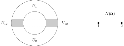
An annulus covered by the upper half and the lower half : the intersection (shaded) consists of two pieces and is not contractible. The nerve is contractible, a segment; the annulus is not.
The theorem applies to our data-analysis scenario: take and cover it by the balls themselves. All finite intersections are intersections of convex sets, and an intersection of convex sets is convex, hence empty or contractible: convexity gives a Leray cover. The nerve of this cover is exactly the Čech complex , and the nerve theorem gives .
The category of covers and paracompactness
There is a word in the theorem that should have frightened you; I will explain it. Who knows what a paracompact space is? The existence of a partition of unity is a theorem; the definition of paracompactness is a little different and is given in terms of covers. For that we need structures on covers: the covers of a given space form a category, not just a partial order.
Definition (Refinement). Let and be two open covers of . is called a refinement of if for every there is an such that .
Whichever member of the second cover you take, it is contained in some member of the first. One would like to introduce a preorder on the set of all covers using the notion of refinement, but is not uniquely determined by , and it is more correct to consider all possible choices of where exactly to put , into or into .
Definition (Category of covers). The category of covers : the objects are the open covers of ; the morphisms from to are all ways of fitting into , that is, maps of the index sets such that for every .
The notion of paracompactness is defined in these terms.
Definition (Paracompactness). A space is paracompact if every open cover of it has a locally finite refinement: one in which every point has a neighbourhood meeting only finitely many members of the cover.
Facts. CW complexes are paracompact; metric spaces are paracompact; these are hard theorems of general topology. If a space is paracompact, every open cover of it has a subordinate partition of unity; this is an easy theorem, usually included in a general topology course. It is exactly the partition of unity that is needed to prove the nerve theorem.
How it is proved. Between and the nerve one builds an auxiliary space: each is multiplied by the corresponding vertex of the nerve, and each intersection by the corresponding simplex :
If is covered by two sets, this is and with the cylinder glued to them. This space has a projection onto and a projection onto the nerve, and one proves that both are homotopy equivalences: a section of the first is built using a partition of unity, a section of the second too, in a certain way. You can read about this in Hatcher, section 4.G; in principle it should be accessible to you.
Two more notions in terms of covers
Lebesgue covering dimension. One says that the topological dimension of a space is at most , , if into any open cover of it one can fit a refinement whose nerve has dimension at most , that is, in which no members have a nonempty common intersection.
Example (the square). The square is compact, so from any cover one can extract a finite subcover; one may assume it consists of balls. Into it one can fit a hexagonal grid of small discs whose nerve is two-dimensional. So the Lebesgue dimension of the square is at most two. In general, the Lebesgue dimension of an -dimensional CW complex is .
Čech homology and cohomology. Eduard Čech was a well-known Czech topologist; the háček on top means "Čech". For each open cover one can compute the simplicial homology of its nerve . When one cover fits into another (there is a morphism ), a simplicial map arises at the level of nerves: a map on vertices, , which extends linearly to the simplices (we have not defined these yet), and it gives a map of homology. Čech homology is defined as the inverse limit over the category of covers:
and Čech cohomology as the direct limit of the corresponding cohomology groups of the nerves. The category of covers is filtered in the classical sense: any two covers have a common refinement.
An example: a cover by three sets whose nerve is a triangle; into it one fits a finer cover whose nerve is some stranger thing. Two of its vertices map to one vertex of the triangle, two more to another, one to the third, and on the remaining simplices the map is extended linearly: the nerve of maps to the nerve of .
If is a good space, Čech homology is isomorphic to singular homology, which our course is about. If is not a very good space, it behaves better than singular homology and suits some questions better, but to work with it one needs the technique of direct and inverse limits. The idea is this: there are very many covers and they are frightening, but in a good space, a locally contractible one, Leray covers form a final subsystem, and one can compute with them; for Čech cohomology a Leray cover then gives the answer at once, while with homology there is the torment of , the derived functor of the inverse limit. This is how one proves that for a locally contractible Hausdorff paracompact space Čech cohomology is isomorphic to singular cohomology.
If all this frightens you, in our course these notions are unlikely to come up again; perhaps I will someday say something about paracompactness, but unlikely.
No comments yet
Be the first to share your thoughts.