September 22, 2026 · Lecture · LibreTimes
Probability Theory. Lecture 1
About the course
This is a fairly standard course in probability theory, with one difference. Usually the course is given when the students are only beginning to learn measure theory and the Lebesgue integral, so it includes a large discrete part in order to postpone the moment when a real probability measure and a real expectation as a Lebesgue integral appear. We will not postpone it: measure and the Lebesgue integral are assumed to be known – not "heard of it", but you know how a measure is constructed, how the integral is constructed, the main theorems on passing to the limit, Fubini's theorem, what an absolutely continuous measure is and the Radon–Nikodym theorem. The first two lectures will not need this (today's lecture is almost school level), but fairly soon it will turn out that you need to know all of it. If you have not had it, most of the course will be hard, and not because of the substance but because of unfamiliarity with the language.
What is usually not in the standard exposition: Kolmogorov's theorem on consistent families; besides Chebyshev's inequality there will be Bernstein's inequality, which is now considered very important in applications; the characteristic function in the context of the Fourier transform, that is, where it comes from, and not just "a strange function with useful properties". There will be a section on convergence (the law of large numbers, convergence of series of independent random variables) and at the end the central limit theorem with various ways of proving it.
Four problem sheets, substantial ones; a written exam. Credit for the sheets: of everything that could be handed in, and not a single empty sheet; the course is credited with the exam grade.
Textbooks on probability theory:
- A. N. Shiryaev. Probability. An excellent textbook, only thick; use it as a book where you find the section you need, not read it cover to cover. Shiryaev also has Problems in Probability, an interesting collection.
- J. Lamperti. Probability. A thin, small-format book that reads like fiction and at the same time covers the main topics; it assumes knowledge of measure and the Lebesgue integral. It was translated in the seventies by S. A. Molchanov, with his appendix.
- W. Feller. An Introduction to Probability Theory and Its Applications, two volumes. An old book, from the middle of the last century, but it contains many topics that are not in other textbooks: later books were written from lectures, and the hard things dropped out of the lectures, while here they are collected; a huge number of worked examples and large problem collections.
- A. Shen. Probability: Examples and Problems (MCCME): a thin booklet for schoolchildren, for those who do not want higher mathematics but want to solve nice problems; the law of large numbers is there, and many historical topics. Whoever solves everything in it has a level of "not bad at all".
What we will use from analysis and measure theory:
- V. I. Bogachev, O. G. Smolyanov. Real and Functional Analysis. I strongly advise everyone to read the first chapter once, and at the same time check what you know from basic analysis; measure theory is chapters 2–4; then functional analysis, which will also be needed (counterexamples via the Hahn–Banach theorem).
- V. I. Bogachev. Measure Theory, two volumes: for special information.
- V. I. Bogachev. Weak Convergence of Measures: towards the end of the course; a small book, roughly like Billingsley's Convergence of Probability Measures, a little more modern.
Also: O. Kallenberg, Foundations of Modern Probability; A. A. Borovkov, Probability Theory; N. Alon, J. Spencer, The Probabilistic Method: on how probability is applied outside probability itself.
The probability space
Let us adopt the following picture of how probability theory arises. There is an experiment that we can, at least in thought, reproduce without changes as many times as we like. The experiment has outcomes. We usually group outcomes; sets of outcomes are called events. To each event we want to assign a number, the probability, and the meaning of this number is to describe how often the event occurs when the experiment is repeated many times.
Probability is about frequency. There is nothing rigorous in this: we hope to build a model in which this will be so, and when we get through the law of large numbers, that will be the moment when we understand that we have built what we wanted. We put nothing more into it.
The part about the experiment does not belong to mathematics; it is as life gives it. From there on, mathematics describes everything.
Definition (Finite probability space). is a finite set, the set of outcomes. An event is any subset of ; the set of events is . A probability (probability measure) is a function
satisfying two conditions:
- ;
- the sum rule: if , then .
Both conditions are natural. If you take all outcomes and add up the frequencies with which they occur, you must get . If events do not intersect (some outcomes here, others there), then the frequency of "at least one of them" is the sum of the frequencies: in experiments outcomes from occurred times, from times, so the union . Literally so.
People say "a probability measure on ", and that is slang; in reality it is defined on .
Five properties of probability
What can be said about such a function, how is it arranged? The following properties help to understand it better. There are five of them, and after them you can consider that you know everything about probability, with proofs.
Let us agree on notation: and denote a union of sets that are pairwise disjoint, so as not to write "pairwise disjoint" every time.
Theorem (Properties of probability). Let be a probability measure on , .
- .
- If , then .
- The inclusion–exclusion formula:
- If the events are pairwise disjoint, then .
- .
Proof. 1. The only thing we can do is the sum rule, so the union has to be written through disjoint sets: , whence . That is not it yet, but , so . Substitute.
2. , so , since probability is nonnegative.
3. Induction on ; for this is property 1. Suppose the formula holds for . Separate the first events and apply property 1:
The first term, by the induction hypothesis, gives all the terms of the formula in which does not take part; the second gives the term ; the third is again a union of events, to which the formula for applies, and it gives (with a change of sign) all the intersections in which takes part. The induction step is done.
4. If the events are disjoint, all the intersections in the inclusion–exclusion formula are empty, and : indeed, , so , which is possible only for zero. The first sum remains.
5. This cannot be seen from the inclusion–exclusion formula: there are pluses and minuses there. But a union in which the events may intersect can always be written as a union without intersections: keep the first, from the second only what is not counted in the first, from the third only what does not belong to the first two, and so on:
The probability is the sum of the probabilities of the pieces, and each piece, starting from the second, is a subset of its , so by property 2 the sum does not exceed .
Remark (why the inclusion–exclusion formula is needed). This formula itself tells you almost everything you need to know when solving problems on computing probabilities. It is useful to split a problem into subproblems, the outcomes you need into smaller events, and the splitting is done by fixing some parameter: "consider the cases where the result of the first throw is such-and-such". The splitting need not be disjoint: split however is convenient. And then there is no need to sit and wonder "have I counted this outcome or not, it seems I multiplied here and counted it, but divided there and did not"; that way you will never know whether you have solved the problem. The scheme is one: divide and rule. Divide into pieces so that they are convenient to count; assemble by this formula. In the intersections even more parameters are fixed, the problem becomes even more concrete, and the further you go, the simpler it is.
All probability measures on a finite set
The five properties mean that we can say everything about .
Theorem (Description of probability measures on a finite set). Let .
- If is a probability measure on , then there are numbers with such that for every
Moreover, .
- Conversely, for any numbers with this formula defines a probability measure on .
Proof. 1. ; the sum rule (property 4) gives the formula with . The numbers are nonnegative since ; the sum of all of them is .
2. Two things need to be checked. Substitute : all the are summed, and we get one. The sum rule: if and do not intersect, then the sets of indices taking part in the formula do not intersect either, and the sum splits in two.
In the finite case there is no mystery in a probability measure: it is a completely clear object, mathematically nothing special. Weights are assigned to the outcomes, and the probability of an event is the sum of the weights of the outcomes that fall into it.
Equally likely outcomes
Definition (Equally likely outcomes). An important special case: all the are equal. Then
the number of outcomes in divided by the number of all outcomes. One says that the outcomes are equally likely.
Equal likelihood is not a self-evident assumption but part of your model. Probability begins after a probability space has appeared: it has been said what is and how probability is assigned to events. Until this has been said, there is nothing to talk about. Solving problems in the style of "well, clearly times , that gives , that is the answer" is no way to talk: there is no science in which numbers are simply multiplied. How the probability space is built determines which numbers to add, which to multiply, and why the answer is what it is.
Example (a die with coloured faces). A die, three faces red, two blue, one yellow. We throw it and look at the colour of the face that comes up. The outcome of the experiment: a colour. There is no mathematics in this yet; it begins when someone says "I want to compute the probability": a probability space must be presented.
Model 1. Three outcomes (red, blue, yellow); the simplest model: equally likely, each. You put the organisation's stamp on it and take it to the client. The client throws a hundred times, red comes up much more often than a third, and comes back: "something is wrong". But where is the mistake? The sum is one, the numbers are nonnegative, the mathematics is fine. What is bad is the model, that is, the contact with the client.
Model 2. Six outcomes (the faces), each; the colours are events: , , . The client throws a while, and it fits.
A priori neither model is better than the other; both have a mathematical right to exist. Which one is right is determined by agreement with the experiment, and this must be written into the statement of the problem: "the faces are equally likely".
Why do we want to reduce a problem to equally likely outcomes? Because it is easier to count: you divide the number you need by the total, combinatorics instead of probability theory. Can this always be done? If equal likelihood is understood a little more broadly, then always, and this will be one of the most remarkable theorems of the course: all reasonable distributions are obtained from the uniform law. In the discrete case this can be seen purely mathematically.
Remark (reduction to equally likely outcomes). Let the probabilities be rational fractions. Bring them to a common denominator : . Pass to a new space of equally likely outcomes in which the old outcome has become an event consisting of new outcomes. There is no meaning behind this transition (unlike the transition from colours to faces), but technically it is always possible. If the probabilities are irrational, they can be approximated by rational ones, and the reduction will be approximate, with a small gap; and if an infinite space of outcomes is allowed, then exact.
Behind this technical point there is an idea: the basic laws of probability can be seen in the equally likely situation (in effect taken from combinatorics, from the ability to count quantities) and used in the general one. The product rule, the law of total probability, Bayes' formula, stated as theorems of probability, in fact express ways of counting proportions. We are entitled to carry them over to a general probability space precisely because we reduce any situation, exactly or approximately, to an equally likely one. This is not a philosophical agreement of the kind "compute conditional probability this way and no other".
Classical paradoxes: the choice of a model
The choice of a model is not obvious. With the die everything is more or less clear, but there are historical examples that were a mystery to people; for a long time they were called paradoxes, because there was no science, it was not understood how a general scheme is built at all. All this is before Kolmogorov, before the axiomatics.
Example (two dice). Two dice are thrown, and the sum of the points is looked at. Which comes up more often, or ? Naively: the sums range from to , all are possible, why should they differ. But in taverns and ports dice were thrown often, and people observed that nine comes up more often. So the model fails to take something into account, for example that there are two dice.
We do the same as with the coloured die: go down to a more primary object, physically more symmetric. An outcome is not the sum, not processed data, but exactly what is observed: the pair of numbers that came up. Then there are equally likely outcomes of each, and
that is, , .
Why not count twice? Because we declared the cells of the table to be the outcomes and took them to be equally likely. "But why are they equally likely, maybe the diagonal has more weight?" Mathematics will not answer that; if the sum is one, everything is in order. The two models are mathematically indistinguishable; the motivation comes from the experiment.
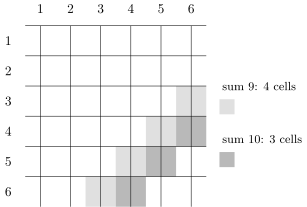
The outcomes are the cells of a table, each. The sum comes from four cells, the sum from three.
Example (the division of the stakes). An ancient problem, fifteenth–sixteenth centuries. A game of heads-or-tails was played to six wins: heads means the first player wins the round, tails the second. Eight rounds were played, the first won five, the second three, and they did not finish. In what proportion should the prize be divided?
The question is not even mathematical. "Five parts to one, three to the other" – but why? "I was unlucky, and now everything will turn around" is also possible.
The first way: finish the game in thought. The ways it could finish: H (the first won at once); TH; TTH; TTT (the second won). Four variants, in three of them the first wins, divide . Some thought this was the right answer.
Then people wondered: what are these cases? In effect they arise if you throw three times, but in the first variant, after heads, the remaining throws "do not count". Hitting the target with the first shot and three times in a row are completely different matters; one does not want to consider these variants equally likely. To build equally likely outcomes one has to assume that the coin was effectively thrown three times (eight outcomes, zeros and ones in three positions), although that is hard to accept: why throw if the game is over? We subdivide the outcomes in order to pass to equally likely ones. Then the variant H is outcomes out of , TH , TTH , TTT : the first wins with probability , the second with , divide . The second player liked the first model better, but this one is more adequate to what we understand by equally likely outcomes.
Different mathematicians gave different answers, and there were disputes over it. The problem sheet has Banach's matchbox problem; there you will have to do the same thing: the matches can run out after different numbers of draws, and the outcomes must be subdivided to a common number.
Example (Bertrand's paradox). This is already an infinite space of outcomes, but the problem is the same, so we will tell it here and not come back to it. At the beginning of the twentieth century this was still a paradox.
A chord is drawn at random in a circle. What is the probability that it is longer than the side of the inscribed regular triangle? The side is fixed; the question is reasonable. But what does "a chord is drawn at random" mean? Here the room for fantasy begins.
- Fix one end of the chord (the situation can always be rotated), and choose the second at random on the circle; the probability is the length of the required set divided by the length of the circle. For the chord to be longer than the side, the second end must fall in the middle third of the arc. The answer is .
- Throw a point into the disc and draw through it the chord perpendicular to the radius. The chord is longer than the side when the point has fallen inside the circle of radius inscribed in the triangle; the probability is the ratio of the areas. The answer is .
- Rotate so that the chord is perpendicular to a given radius, and choose at random a point on the radius, the midpoint of the chord. It must fall in the half of the radius nearer the centre. The answer is .
All three answers are reasonable. Which is right? The question is meaningless: from the point of view of mathematics they are all fine. Want to know which is right? Experiment. The disputes went on until it was realised that there was nothing to dispute: mathematicians can argue only after a probability space has been fixed, and here there are three different ones: a point on a circle, a point in a disc, a point on a segment.
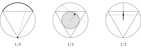
Three probability spaces for a "random chord": the second end on the circle (the middle third of the arc is needed), the midpoint of the chord in the disc (the disc of radius is needed), the midpoint of the chord on a radius (its half is needed).
It may seem that one of the variants is "more correct", say two points thrown uniformly on the circle. But correct for whom? There are differences between the variants; for example, the distribution of the midpoint of the chord in variants 2 and 3 is different, which is the same difference as when passing to polar coordinates, where one has to multiply by . But that is a question about the distribution of a point, while we are discussing the distribution of a chord, which is built in a more complicated way. Why one difference should say that one variant is worse than another is unclear. Only experiment can stand behind the answer to all this.
Conditional probability
Let a probability measure, not necessarily equally likely, be given on .
Definition (Conditional probability). Let . The conditional probability of the event given is
This is a definition; you may like it or not. The meaning we want to put into it: the probability of if it is already known that only outcomes from take place. The formula is motivated through equally likely outcomes. If all outcomes are equally likely, . If it is known that has happened, the experiment ends only in results from , and among themselves they are still indistinguishable; so one must divide the number of outcomes of belonging to by the number of outcomes of . We have renormalised: before, an outcome weighed , now , and the outcomes are as equally likely as they were. In other words,
that is, the conditional probability is the proportion of among . Only we do not want to say it that way, and for some reason say "conditional probability". And then we take this rule and declare: let it now always be so. The transition is adequate because the general situation can be reduced to an equally likely one, the motivated formula taken from there, and we can come back.
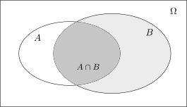
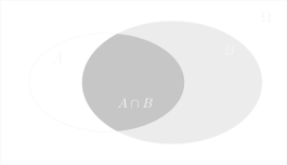
is the proportion of the dark part in the light one: once is known, the outcomes outside are discarded and the remaining ones renormalised.
The formula is immediately rewritten as
and called the product rule. For equally likely outcomes this is the ordinary rule for computing proportions taught in primary school: to find what proportion of the whole the piece of belonging to makes up, multiply the proportion of by the proportion of this piece within .
Example (two balls without replacement). A box has balls, of them white. Two balls are drawn without replacement; what is the probability that both are white? Many start like this: the first is white with probability ; if a white one was drawn, there is one white fewer and one ball fewer in total, giving ; multiply. But where is the probability theory here?
In fact you subconsciously go through the whole path. You declared the ordered pairs of drawn balls to be the outcomes and took them to be equally likely, so you compute probabilities as proportions. Among all pairs, the proportion of those whose first ball is white is . Within each "row" with a fixed white first ball, the proportion of pairs with a white second ball is , and this proportion is the same in all rows, so it is the same in the whole set. In one formula, without telling anyone anything, you introduced a probability space, declared the outcomes equally likely, carried out a not entirely obvious computation with proportions, and called it the product rule. That is allowed, but when you hand in the first sheet you will have to say it all: which space, why equally likely. If the outcomes are not equally likely, you cannot compute with proportions.
Remark (a vicious circle). In a concrete problem the conditional probability is defined through the probability of the intersection, while the probability of the intersection is computed by the product rule through the conditional one – the wind blows because the trees sway. When you multiply " by ", where did you get the conditional probability from? By definition, for that you had to compute the intersection. You do it by appealing to the equally likely situation and forgetting all of probability theory: you just count proportions. The purpose of this discussion of elementary probability is to drive home the understanding that behind every step there is a definite logic, not a philosophical agreement.
In many problems conditional probabilities are given a priori. The question arises: is there a probability measure for which they are the conditional probabilities? Where did you get the idea that there always is one? The answer is given by the following formula.
The law of total probability
Theorem (Law of total probability). Let , . Then for every event
Proof. by the sum rule, and each intersection, by the product rule, equals . It is no more than the sum rule coordinated with the definition of conditional probability.
The formula not only lets us compute but also explains something. A typical situation in genre problems: two firms sell computers, one has such a probability of a defect, the other such, the firms' market shares are known; you bought a computer; what is the probability of a defect? By the law of total probability, and everything seems clear. But what happened? All outcomes were split into two parts, positive numbers summing to one were assigned to the parts, and within each part its own probability was introduced. And where did you get the idea that the problem makes sense, that a probability measure exists for these data? The catch in such problems is that the probability space is not given in them; its existence somewhere out in space has to be taken on faith.
Theorem (A measure from conditional probabilities). Let ; let numbers with and probability measures on with be given (that is, outside the measure is zero). Then there is a unique probability measure on for which
Proof. Put
This is a probability measure: for all and the sum equals ; the sum rule holds for each term. Feed in : all terms except the -th vanish, since for , and the -th gives . The conditional probability:
since kills all terms except the -th, and itself takes from only the part lying in . Uniqueness follows from the law of total probability: the measure of any is determined by the conditional probabilities and the probabilities of the conditions.
Problems in which the probabilities of the conditions and the conditional probabilities are given are indeed well posed: from these data the probability measure is recovered. The law of total probability is the second way of defining a probability. The first: assign a weight to each outcome; the second: split the space into parts, give the probabilities of the parts and a probability measure within each, and assemble the measure by the law of total probability. So the formula is not a trivial application of the sum rule but a very important observation.
Bayes' formula
Theorem (Bayes' formula). Let , . Then
Proof. The probability of the intersection is written in two ways: . That is the whole proof.
Probability is a romantic science, with beautiful names invented for things, starting with the word itself. You listen: "you knew the probability of given , and you can find out the probability of given ; the condition and the event swap places"; it sounds like science fiction. But if you approach it mercenarily, as counting proportions, it is a trivial thing: the proportion of among and the proportion of among are computed through one and the same thing, , only renormalised by or by . That is all there is to Bayes' formula. Some of you are disappointed.
Example (a classifier). From here on everything depends on how corrupted you are; from here on it is marketing: anyone could do a simple thing, but not everyone can sell it. A machine must be taught, on seeing a person, to greet them with "hello, mathematician" or "hello, physicist". The machine looks at height, build, asks questions ("what is two times two", "does a brick sink") and must draw a conclusion from the answers; deterministically this cannot be decided from such a list. What it knows: the proportion of mathematicians and of physicists in general, and the proportion of such answers among mathematicians and among physicists. It needs the reverse: how many mathematicians there are among all who answered this way, and how many physicists. Whoever is more numerous among those who answered this way, that is probably what the person is. A natural thing; told like this, it sounds too simple. Or one can tell it like this: "we apply Bayes' formula, compute the reverse probabilities, compare with ".
There is no secret science behind the formula, accessible only to the chosen; it is the ordinary calculus of proportions carried over to the general situation. That is what makes it remarkable: it is correct not only because we derived it from the definition but because it is true for ordinary counting of quantities. That is why we believe in it.
Independence
So far the whole discussion has been about the calculus of quantities and proportions, which for some reason we beautifully call probability; if that were all, it would be a strange discussion of combinatorics. Real probability theory begins when the notion of independence is introduced. It is independence that makes probability out of combinatorics and measure theory; without it, these are simply chapters of discrete mathematics or of measure and integration theory.
Definition (Independence of two events). Events and are independent if
A beautiful symmetric definition and a beautiful word. But what does not depend on what? With vectors it is clear: one is expressed through the other, so they are dependent. Here independence is in a different sense: not that one quantity depends on another, but in the sense of influence on the calculation of probabilities. If , the definition is equivalent to
the proportion of among is the same as among everything.
This leads to sad thoughts: independence does not happen at all. Is the fact that you like ice cream dependent on the fact that you go to the Independent University? Most likely it is dependent: the proportion of ice-cream lovers at the IUM is unlikely to coincide with the proportion on the whole planet. Independence is an extremely rigid restriction.
Example (divisibility by and by). One number is chosen from the first , all equally likely. : it is divisible by , : it is divisible by . The proportion divisible by is , by is , by is :
Independent. Now take the first numbers. The number is divisible neither by nor by ; it does not affect anything. But the proportions have become , , , and
By definition, dependent. There is no intuition here at all: it would be one thing if a number divisible by had been added, but the addition was harmless to both events.
Independence as an equality of proportions: it is very strange to think that such a thing should be observed in life. In studying independent events you have moved into an abstraction, an ideal situation; the assumption of independence is an idealisation, a mathematical model, and not something self-evident. If the problem statement does not say that the events are independent and you are going to multiply the probabilities, that is your problem, and you must explain why they are independent.
Next time, more about what independence of events means.
No comments yet
Be the first to share your thoughts.